Quantify dataset - examples#
See also
The complete source code of this tutorial can be found in
In this page we explore a series of datasets that comply with the Quantify dataset specification.
2D dataset example#
We use the mk_two_qubit_chevron_dataset()
to generate our exemplary dataset. Its source code is conveniently displayed in the
drop-down below.
dataset = dataset_examples.mk_two_qubit_chevron_dataset()

assert dataset == round_trip_dataset(dataset)  # confirm read/write
dataset
<xarray.Dataset> Size: 115kB
Dimensions:  (repetitions: 5, main_dim: 1200)
Coordinates:
    amp      (main_dim) float64 10kB 0.45 0.4534 0.4569 ... 0.5431 0.5466 0.55
    time     (main_dim) float64 10kB 0.0 0.0 0.0 0.0 ... 1e-07 1e-07 1e-07 1e-07
Dimensions without coordinates: repetitions, main_dim
Data variables:
    pop_q0   (repetitions, main_dim) float64 48kB 0.5 0.5 0.5 ... 0.4818 0.5
    pop_q1   (repetitions, main_dim) float64 48kB 0.5 0.5 0.5 ... 0.5371 0.5
Attributes:
    tuid:                      20250904-040830-272-541b86
    dataset_name:
    dataset_state:             None
    timestamp_start:           None
    timestamp_end:             None
    quantify_dataset_version:  2.0.0
    software_versions:         {}
    relationships:             []
json_serialize_exclude: []The data within this dataset can be easily visualized using xarray facilities,
however, we first need to convert the Quantify dataset to a “gridded” version with the to_gridded_dataset() function as
shown below.
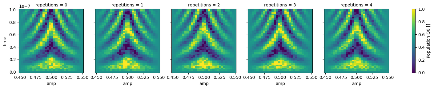
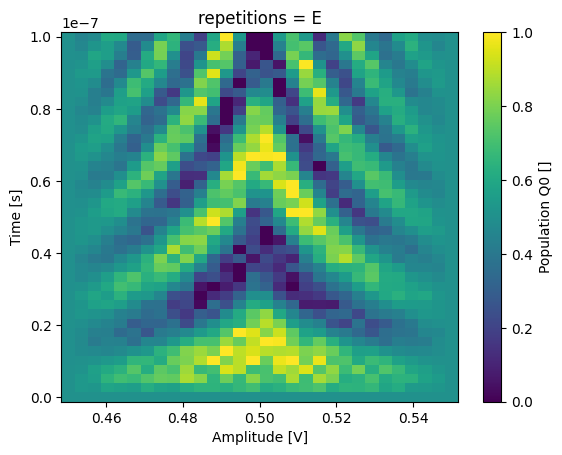
Since our dataset contains multiple repetitions of the same experiment, it is convenient to visualize them on different plots.
dataset_gridded = dh.to_gridded_dataset(
dataset,
dimension="main_dim",
coords_names=dattrs.get_main_coords(dataset),
)
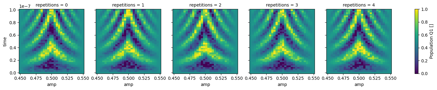
dataset_gridded.pop_q0.plot.pcolormesh(x="amp", col="repetitions")
_ = dataset_gridded.pop_q1.plot.pcolormesh(x="amp", col="repetitions")
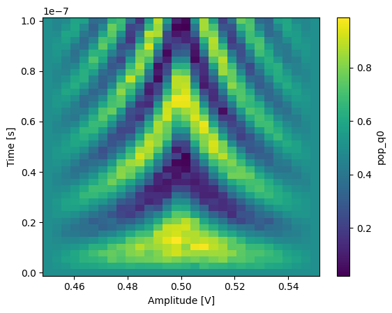
In xarray, among other features, it is possible to average along a dimension which can be very convenient to average out some of the noise:
_ = dataset_gridded.pop_q0.mean(dim="repetitions").plot(x="amp")
A repetitions dimension can be indexed by a coordinate such that we can have some specific label for each of our repetitions. To showcase this, we will modify the previous dataset by merging it with a dataset containing the relevant extra information.
coord_dims = ("repetitions",)
coord_values = ["A", "B", "C", "D", "E"]
dataset_indexed_rep = xr.Dataset(coords=dict(repetitions=(coord_dims, coord_values)))

dataset_indexed_rep
<xarray.Dataset> Size: 20B
Dimensions:      (repetitions: 5)
Coordinates:
  * repetitions  (repetitions) <U1 20B 'A' 'B' 'C' 'D' 'E'
Data variables:
*empty*# merge with the previous dataset
dataset_rep = dataset_gridded.merge(dataset_indexed_rep, combine_attrs="drop_conflicts")
assert dataset_rep == round_trip_dataset(dataset_rep) # confirm read/write
dataset_rep
<xarray.Dataset> Size: 97kB
Dimensions:      (amp: 30, time: 40, repetitions: 5)
Coordinates:
  * amp          (amp) float64 240B 0.45 0.4534 0.4569 ... 0.5431 0.5466 0.55
  * time         (time) float64 320B 0.0 2.564e-09 5.128e-09 ... 9.744e-08 1e-07
  * repetitions  (repetitions) <U1 20B 'A' 'B' 'C' 'D' 'E'
Data variables:
    pop_q0       (repetitions, amp, time) float64 48kB 0.5 0.5 0.5 ... 0.5 0.5
    pop_q1       (repetitions, amp, time) float64 48kB 0.5 0.5 0.5 ... 0.5 0.5
Attributes:
    tuid:                      20250904-040830-272-541b86
    dataset_name:
    dataset_state:             None
    timestamp_start:           None
    timestamp_end:             None
    quantify_dataset_version:  2.0.0
    software_versions:         {}
    relationships:             []
json_serialize_exclude: []Now we can select a specific repetition by its coordinate, in this case a string label.
_ = dataset_rep.pop_q0.sel(repetitions="E").plot(x="amp")
T1 dataset examples#
The T1 experiment is one of the most common quantum computing experiments. Here we explore how the datasets for such an experiment, for a transmon qubit, can be stored using the Quantify dataset with increasing levels of data detail.
We start with the most simple format that contains only processed (averaged) measurements and finish with a dataset containing the raw digitized signals from the transmon readout during a T1 experiment.
We use a few auxiliary functions to generate, manipulate and plot the data of the examples that follow:
Below you can find the source-code of the most important ones and a few usage examples in order to gain some intuition for the mock data.
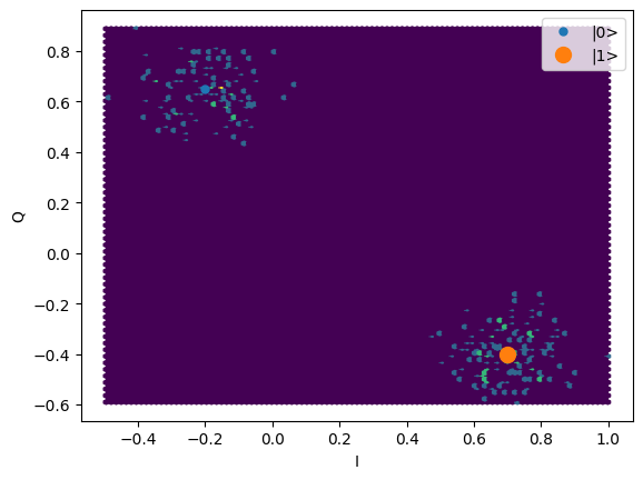
ground = -0.2 + 0.65j
excited = 0.7 - 0.4j
centers = ground, excited
sigmas = [0.1] * 2

shots = mk_iq_shots(
    num_shots=256,
    sigmas=sigmas,
    centers=centers,
    probabilities=[0.4, 1 - 0.4],
)

plt.hexbin(shots.real, shots.imag)
plt.xlabel("I")
plt.ylabel("Q")
_ = plot_complex_points(centers, ax=plt.gca())
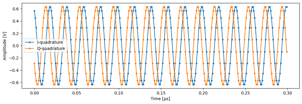
time = mk_trace_time()
trace = mk_trace_for_iq_shot(shots[0])

fig, ax = plt.subplots(1, 1, figsize=(12, 12 / 1.61 / 2))
ax.plot(time * 1e6, trace.imag, ".-", label="I-quadrature")
ax.plot(time * 1e6, trace.real, ".-", label="Q-quadrature")
ax.set_xlabel("Time [µs]")
ax.set_ylabel("Amplitude [V]")
_ = ax.legend()
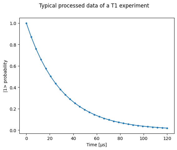
First, we define a few parameters of our mock qubit and mock data acquisition.
# parameters of our qubit model
tau = 30e-6
ground = -0.2 + 0.65j  # ground state on the IQ-plane
excited = 0.7 - 0.4j  # excited state on the IQ-plane
centers = ground, excited
sigmas = [0.1] * 2  # sigma, NB in general not the same for both state

# mock of data acquisition configuration
# NB usually at least 1000+ shots are taken, here we use less for faster code execution
num_shots = 256
# time delays between exciting the qubit and measuring its state
t1_times = np.linspace(0, 120e-6, 30)

# NB this are the ideal probabilities from repeating the measurement many times for a
# qubit with a lifetime given by tau
probabilities = exp_decay_func(t=t1_times, tau=tau, offset=0, n_factor=1, amplitude=1)

# Ideal experiment result
plt.ylabel("|1> probability")
plt.suptitle("Typical processed data of a T1 experiment")
plt.plot(t1_times * 1e6, probabilities, ".-")
_ = plt.xlabel("Time [µs]")
# convenience dict with the mock parameters
mock_conf = dict(
    num_shots=num_shots,
    centers=centers,
    sigmas=sigmas,
    t1_times=t1_times,
    probabilities=probabilities,
)
T1 experiment averaged#
In this first example, we generate the individual measurement shots and average them, similar to what some instruments are capable of doing directly in the hardware.
Here is how we store this data in the dataset along with the coordinates of these datapoints:
dataset = dataset_examples.mk_t1_av_dataset(**mock_conf)
assert dataset == round_trip_dataset(dataset)  # confirm read/write

dataset
<xarray.Dataset> Size: 720B
Dimensions:   (main_dim: 30)
Coordinates:
    t1_time   (main_dim) float64 240B 0.0 4.138e-06 ... 0.0001159 0.00012
Dimensions without coordinates: main_dim
Data variables:
    q0_iq_av  (main_dim) complex128 480B (-0.19894114958423859+0.651550013884...
Attributes:
    tuid:                      20250904-040832-948-fbb6ac
    dataset_name:
    dataset_state:             None
    timestamp_start:           None
    timestamp_end:             None
    quantify_dataset_version:  2.0.0
    software_versions:         {}
    relationships:             []
json_serialize_exclude: []dataset.q0_iq_av.shape, dataset.q0_iq_av.dtype
((30,), dtype('complex128'))
dataset_gridded = dh.to_gridded_dataset(
    dataset,
    dimension="main_dim",
    coords_names=dattrs.get_main_coords(dataset),
)
dataset_gridded
<xarray.Dataset> Size: 720B
Dimensions:   (t1_time: 30)
Coordinates:
  * t1_time   (t1_time) float64 240B 0.0 4.138e-06 ... 0.0001159 0.00012
Data variables:
    q0_iq_av  (t1_time) complex128 480B (-0.19894114958423859+0.6515500138845...
Attributes:
    tuid:                      20250904-040832-948-fbb6ac
    dataset_name:
    dataset_state:             None
    timestamp_start:           None
    timestamp_end:             None
    quantify_dataset_version:  2.0.0
    software_versions:         {}
    relationships:             []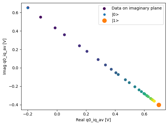
json_serialize_exclude: []plot_xr_complex(dataset_gridded.q0_iq_av)
fig, ax = plot_xr_complex_on_plane(dataset_gridded.q0_iq_av)
_ = plot_complex_points(centers, ax=ax)

T1 experiment averaged with calibration points#
It is common for many experiments to require calibration data in order to interpret the results. Often, these calibration data points have different array shapes. E.g. it can be just two simple data points corresponding to the ground and excited states of our transmon.
To accommodate this data in the dataset we make use of a secondary dimension along which the variables and its coordinate will lie along.
Additionally, since the secondary variable and coordinate used for calibration can have
arbitrary names and relate to other variables in more complex ways, we specify this
relationship in the dataset attributes
(see QDatasetIntraRelationship).
This information can be used later, for example, to run an appropriate analysis on this
dataset.
dataset = dataset_examples.mk_t1_av_with_cal_dataset(**mock_conf)
assert dataset == round_trip_dataset(dataset)  # confirm read/write

dataset
<xarray.Dataset> Size: 776B
Dimensions:       (main_dim: 30, cal_dim: 2)
Coordinates:
    t1_time       (main_dim) float64 240B 0.0 4.138e-06 ... 0.0001159 0.00012
    cal           (cal_dim) <U3 24B '|0>' '|1>'
Dimensions without coordinates: main_dim, cal_dim
Data variables:
    q0_iq_av      (main_dim) complex128 480B (-0.19894114958423859+0.65155001...
    q0_iq_av_cal  (cal_dim) complex128 32B (0.7010588504157614-0.398449986115...
Attributes:
    tuid:                      20250904-040833-426-8cdf27
    dataset_name:
    dataset_state:             None
    timestamp_start:           None
    timestamp_end:             None
    quantify_dataset_version:  2.0.0
    software_versions:         {}
    relationships:             [{'item_name': 'q0_iq_av', 'relation_type': 'c...
json_serialize_exclude: []dattrs.get_main_dims(dataset), dattrs.get_secondary_dims(dataset)
(['main_dim'], ['cal_dim'])
dataset.relationships
[
    {
        'item_name': 'q0_iq_av',
        'relation_type': 'calibration',
        'related_names': ['q0_iq_av_cal'],
        'relation_metadata': {}
    }
]
As before the coordinates can be set to index the variables that lie along the same dimensions:
dataset_gridded = dh.to_gridded_dataset(
    dataset,
    dimension="main_dim",
    coords_names=dattrs.get_main_coords(dataset),
)
dataset_gridded = dh.to_gridded_dataset(
    dataset_gridded,
    dimension="cal_dim",
    coords_names=dattrs.get_secondary_coords(dataset_gridded),
)
dataset_gridded
<xarray.Dataset> Size: 776B
Dimensions:       (t1_time: 30, cal: 2)
Coordinates:
  * t1_time       (t1_time) float64 240B 0.0 4.138e-06 ... 0.0001159 0.00012
  * cal           (cal) <U3 24B '|0>' '|1>'
Data variables:
    q0_iq_av      (t1_time) complex128 480B (-0.19894114958423859+0.651550013...
    q0_iq_av_cal  (cal) complex128 32B (0.7010588504157614-0.3984499861154196...
Attributes:
    tuid:                      20250904-040833-426-8cdf27
    dataset_name:
    dataset_state:             None
    timestamp_start:           None
    timestamp_end:             None
    quantify_dataset_version:  2.0.0
    software_versions:         {}
    relationships:             [{'item_name': 'q0_iq_av', 'relation_type': 'c...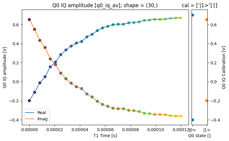
json_serialize_exclude: []fig = plt.figure(figsize=(8, 5))
ax = plt.subplot2grid((1, 10), (0, 0), colspan=9, fig=fig)
plot_xr_complex(dataset_gridded.q0_iq_av, ax=ax)
ax_calib = plt.subplot2grid((1, 10), (0, 9), colspan=1, fig=fig, sharey=ax)
for i, color in zip(
range(2), ["C0", "C1"]
): # plot each calibration point with same color
dataset_gridded.q0_iq_av_cal.real[i : i + 1].plot.line(
marker="o", ax=ax_calib, linestyle="", color=color
)
dataset_gridded.q0_iq_av_cal.imag[i : i + 1].plot.line(
marker="o", ax=ax_calib, linestyle="", color=color
)
ax_calib.yaxis.set_label_position("right")
ax_calib.yaxis.tick_right()
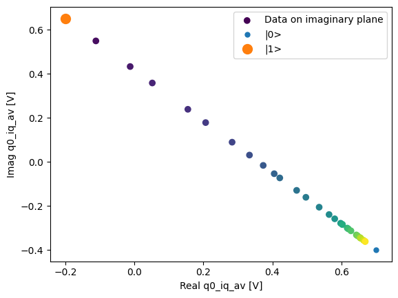
fig, ax = plot_xr_complex_on_plane(dataset_gridded.q0_iq_av)
_ = plot_complex_points(dataset_gridded.q0_iq_av_cal.values, ax=ax)
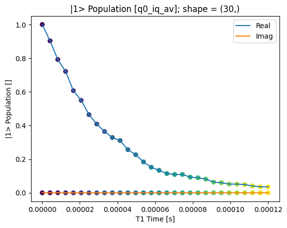
We can use the calibration points to normalize the data and obtain the typical T1 decay.
Data rotation and normalization utilities#
The normalization of the calibration points can be achieved as follows.
Several of the
single-qubit time-domain analyses
provided use this under the hood.
The result is that most of the information will now be contained within the same
quadrature.
rotated_and_normalized = rotate_to_calibrated_axis(
    dataset_gridded.q0_iq_av.values, *dataset_gridded.q0_iq_av_cal.values
)
rotated_and_normalized_da = xr.DataArray(dataset_gridded.q0_iq_av)
rotated_and_normalized_da.values = rotated_and_normalized
rotated_and_normalized_da.attrs["long_name"] = "|1> Population"
rotated_and_normalized_da.attrs["units"] = ""
_ = plot_xr_complex(rotated_and_normalized_da)
T1 experiment storing all shots#
Now we will include in the dataset all the single qubit states (shot) for each individual measurement.
dataset = dataset_examples.mk_t1_shots_dataset(**mock_conf)
dataset
<xarray.Dataset> Size: 132kB
Dimensions:          (main_dim: 30, cal_dim: 2, repetitions: 256)
Coordinates:
    t1_time          (main_dim) float64 240B 0.0 4.138e-06 ... 0.0001159 0.00012
    cal              (cal_dim) <U3 24B '|0>' '|1>'
Dimensions without coordinates: main_dim, cal_dim, repetitions
Data variables:
    q0_iq_av         (main_dim) complex128 480B (-0.19894114958423859+0.65155...
    q0_iq_av_cal     (cal_dim) complex128 32B (0.7010588504157614-0.398449986...
    q0_iq_shots      (repetitions, main_dim) complex128 123kB (-0.28983654535...
    q0_iq_shots_cal  (repetitions, cal_dim) complex128 8kB (0.610163454644259...
Attributes:
    tuid:                      20250904-040834-190-6dd6ac
    dataset_name:
    dataset_state:             None
    timestamp_start:           None
    timestamp_end:             None
    quantify_dataset_version:  2.0.0
    software_versions:         {}
    relationships:             [{'item_name': 'q0_iq_av', 'relation_type': 'c...
json_serialize_exclude: []dataset_gridded = dh.to_gridded_dataset(
dataset,
dimension="main_dim",
coords_names=dattrs.get_main_coords(dataset),
)
dataset_gridded = dh.to_gridded_dataset(
dataset_gridded,
dimension="cal_dim",
coords_names=dattrs.get_secondary_coords(dataset_gridded),
)
dataset_gridded
<xarray.Dataset> Size: 132kB
Dimensions:          (t1_time: 30, cal: 2, repetitions: 256)
Coordinates:
  * t1_time          (t1_time) float64 240B 0.0 4.138e-06 ... 0.0001159 0.00012
  * cal              (cal) <U3 24B '|0>' '|1>'
Dimensions without coordinates: repetitions
Data variables:
    q0_iq_av         (t1_time) complex128 480B (-0.19894114958423859+0.651550...
    q0_iq_av_cal     (cal) complex128 32B (0.7010588504157614-0.3984499861154...
    q0_iq_shots      (repetitions, t1_time) complex128 123kB (-0.289836545355...
    q0_iq_shots_cal  (repetitions, cal) complex128 8kB (0.610163454644259-0.4...
Attributes:
    tuid:                      20250904-040834-190-6dd6ac
    dataset_name:
    dataset_state:             None
    timestamp_start:           None
    timestamp_end:             None
    quantify_dataset_version:  2.0.0
    software_versions:         {}
    relationships:             [{'item_name': 'q0_iq_av', 'relation_type': 'c...
json_serialize_exclude: []In this dataset we have both the averaged values and all the shots. The averaged values can be plotted in the same way as before.
_ = plot_xr_complex(dataset_gridded.q0_iq_av)
_, ax = plot_xr_complex_on_plane(dataset_gridded.q0_iq_av)
_ = plot_complex_points(dataset_gridded.q0_iq_av_cal.values, ax=ax)
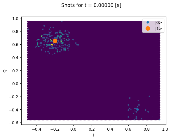
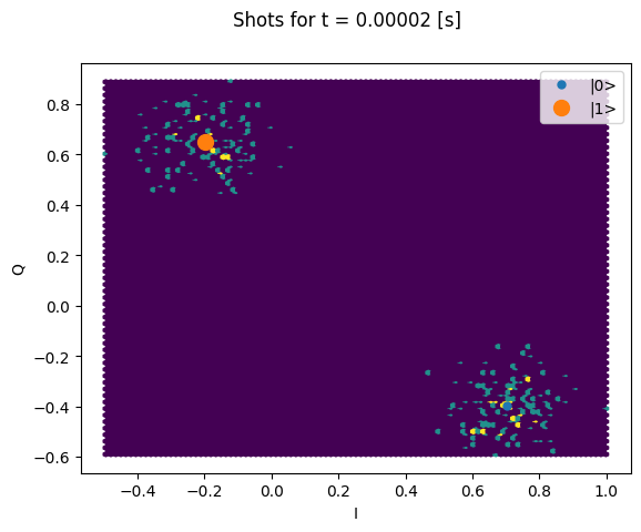
Here we focus on inspecting how the individual shots are distributed on the IQ plane
for some particular Time values.
Note that we are plotting the calibration points as well.
chosen_time_values = [
    t1_times[1],  # second value selected otherwise we won't see both centers
    t1_times[len(t1_times) // 5],  # a value close to the end of the experiment
]
for t_example in chosen_time_values:
    shots_example = (
        dataset_gridded.q0_iq_shots.real.sel(t1_time=t_example),
        dataset_gridded.q0_iq_shots.imag.sel(t1_time=t_example),
    )
    plt.hexbin(*shots_example)
    plt.xlabel("I")
    plt.ylabel("Q")
    calib_0 = dataset_gridded.q0_iq_av_cal.sel(cal="|0>")
    calib_1 = dataset_gridded.q0_iq_av_cal.sel(cal="|1>")
    plot_complex_points([calib_0, calib_1], ax=plt.gca())
    plt.suptitle(f"Shots for t = {t_example:.5f} [s]")
    plt.show()
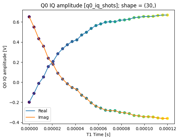
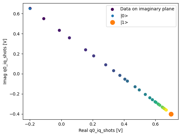
We can collapse (average along) the repetitions dimension:
q0_iq_shots_mean = dataset_gridded.q0_iq_shots.mean(dim="repetitions", keep_attrs=True)
plot_xr_complex(q0_iq_shots_mean)
_, ax = plot_xr_complex_on_plane(q0_iq_shots_mean)
_ = plot_complex_points(centers, ax=ax)
T1 experiment storing digitized signals for all shots#
Finally, in addition to the individual shots we will store all the digitized readout signals that are required to obtain the previous measurement results.
dataset = dataset_examples.mk_t1_traces_dataset(**mock_conf)
assert dataset == round_trip_dataset(dataset)  # confirm read/write

dataset
<xarray.Dataset> Size: 39MB
Dimensions:          (main_dim: 30, cal_dim: 2, repetitions: 256, trace_dim: 300)
Coordinates:
    t1_time          (main_dim) float64 240B 0.0 4.138e-06 ... 0.0001159 0.00012
    cal              (cal_dim) <U3 24B '|0>' '|1>'
    trace_time       (trace_dim) float64 2kB 0.0 1e-09 ... 2.98e-07 2.99e-07
Dimensions without coordinates: main_dim, cal_dim, repetitions, trace_dim
Data variables:
    q0_iq_av         (main_dim) complex128 480B (-0.19894114958423859+0.65155...
    q0_iq_av_cal     (cal_dim) complex128 32B (0.7010588504157614-0.398449986...
    q0_iq_shots      (repetitions, main_dim) complex128 123kB (-0.28983654535...
    q0_iq_shots_cal  (repetitions, cal_dim) complex128 8kB (0.610163454644259...
    q0_traces        (repetitions, main_dim, trace_dim) complex128 37MB (-0.2...
    q0_traces_cal    (repetitions, cal_dim, trace_dim) complex128 2MB (0.6101...
Attributes:
    tuid:                      20250904-040835-626-78125c
    dataset_name:
    dataset_state:             None
    timestamp_start:           None
    timestamp_end:             None
    quantify_dataset_version:  2.0.0
    software_versions:         {}
    relationships:             [{'item_name': 'q0_iq_av', 'relation_type': 'c...
json_serialize_exclude: []dataset.q0_traces.shape, dataset.q0_traces_cal.shape
((256, 30, 300), (256, 2, 300))
dataset_gridded = dh.to_gridded_dataset(
    dataset,
    dimension="main_dim",
    coords_names=["t1_time"],
)
dataset_gridded = dh.to_gridded_dataset(
    dataset_gridded,
    dimension="cal_dim",
    coords_names=["cal"],
)
dataset_gridded = dh.to_gridded_dataset(
    dataset_gridded, dimension="trace_dim", coords_names=["trace_time"]
)
dataset_gridded
<xarray.Dataset> Size: 39MB
Dimensions:          (t1_time: 30, cal: 2, repetitions: 256, trace_time: 300)
Coordinates:
  * t1_time          (t1_time) float64 240B 0.0 4.138e-06 ... 0.0001159 0.00012
  * cal              (cal) <U3 24B '|0>' '|1>'
  * trace_time       (trace_time) float64 2kB 0.0 1e-09 ... 2.98e-07 2.99e-07
Dimensions without coordinates: repetitions
Data variables:
    q0_iq_av         (t1_time) complex128 480B (-0.19894114958423859+0.651550...
    q0_iq_av_cal     (cal) complex128 32B (0.7010588504157614-0.3984499861154...
    q0_iq_shots      (repetitions, t1_time) complex128 123kB (-0.289836545355...
    q0_iq_shots_cal  (repetitions, cal) complex128 8kB (0.610163454644259-0.4...
    q0_traces        (repetitions, t1_time, trace_time) complex128 37MB (-0.2...
    q0_traces_cal    (repetitions, cal, trace_time) complex128 2MB (0.6101634...
Attributes:
    tuid:                      20250904-040835-626-78125c
    dataset_name:
    dataset_state:             None
    timestamp_start:           None
    timestamp_end:             None
    quantify_dataset_version:  2.0.0
    software_versions:         {}
    relationships:             [{'item_name': 'q0_iq_av', 'relation_type': 'c...
json_serialize_exclude: []dataset_gridded.q0_traces.shape, dataset_gridded.q0_traces.dims
((256, 30, 300), ('repetitions', 't1_time', 'trace_time'))
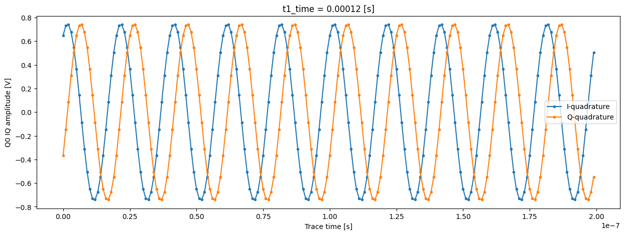
All the previous data is also present, but in this dataset we can inspect the IQ signal for each individual shot. Let’s inspect the signal of shot number 123 of the last “point” of the T1 experiment:
trace_example = dataset_gridded.q0_traces.sel(
    repetitions=123, t1_time=dataset_gridded.t1_time[-1]
)
trace_example.shape, trace_example.dtype
((300,), dtype('complex128'))
Now we can plot these digitized signals for each quadrature. For clarity, we plot only part of the signal.
trace_example_plt = trace_example[:200]
trace_example_plt.real.plot(figsize=(15, 5), marker=".", label="I-quadrature")
trace_example_plt.imag.plot(marker=".", label="Q-quadrature")
plt.gca().legend()
plt.show()