quantify_scheduler.visualization.circuit_diagram

Plotting functions used in the visualization backend of the sequencer.

Module Contents

Functions

gate_box(ax, time, qubit_idxs, text, **kw)	A box for a single gate containing a label.
pulse_baseband(ax, time, qubit_idxs, text, **kw)	Adds a visual indicator for a Baseband pulse to the mathplotlib.axes.Axis
pulse_modulated(ax, time, qubit_idxs, text, **kw)	Adds a visual indicator for a Modulated pulse to the mathplotlib.axes.Axis
meter(ax, time, qubit_idxs, text, **kw)	A simple meter to depict a measurement.
acq_meter(ax, time, qubit_idxs, text, **kw)	Variation of the meter to depict a acquisition.
acq_meter_text(ax, time, qubit_idxs, text, **kw)	Same as acq_meter, but also displays text.
cnot(ax, time, qubit_idxs, text, **kw)	Markers to denote a CNOT gate between two qubits.
cz(ax, time, qubit_idxs, text, **kw)	Markers to denote a CZ gate between two qubits.
reset(ax, time, qubit_idxs, text, **kw)	A broken line to denote qubit initialization.
_locate_qubit_in_address(qubit_map, address)	Returns the name of a qubit in a pulse address.
circuit_diagram_matplotlib(...)	Creates a circuit diagram visualization of a schedule using matplotlib.

gate_box(ax: matplotlib.axes.Axes, time: float, qubit_idxs: List[int], text: str, **kw)

A box for a single gate containing a label.

Parameters:

• ax –

• time –

• qubit_idxs –

• text –

pulse_baseband(ax: matplotlib.axes.Axes, time: float, qubit_idxs: List[int], text: str, **kw)

Adds a visual indicator for a Baseband pulse to the mathplotlib.axes.Axis instance.

Parameters:

• ax –

• time –

• qubit_idxs –

• text –

pulse_modulated(ax: matplotlib.axes.Axes, time: float, qubit_idxs: List[int], text: str, **kw)

Adds a visual indicator for a Modulated pulse to the mathplotlib.axes.Axis instance.

Parameters:

• ax –

• time –

• qubit_idxs –

• text –

meter(ax: matplotlib.axes.Axes, time: float, qubit_idxs: List[int], text: str, **kw)

A simple meter to depict a measurement.

Parameters:

• ax –

• time –

• qubit_idxs –

• text –

acq_meter(ax: matplotlib.axes.Axes, time: float, qubit_idxs: List[int], text: str, **kw)

Variation of the meter to depict a acquisition.

Parameters:

• ax –

• time –

• qubit_idxs –

• text –

acq_meter_text(ax: matplotlib.axes.Axes, time: float, qubit_idxs: List[int], text: str, **kw)

Same as acq_meter, but also displays text.

Parameters:

• ax –

• time –

• qubit_idxs –

• text –

cnot(ax: matplotlib.axes.Axes, time: float, qubit_idxs: List[int], text: str, **kw)

Markers to denote a CNOT gate between two qubits.

Parameters:

• ax –

• time –

• qubit_idxs –

• text –

cz(ax: matplotlib.axes.Axes, time: float, qubit_idxs: List[int], text: str, **kw)

Markers to denote a CZ gate between two qubits.

Parameters:

• ax –

• time –

• qubit_idxs –

• text –

reset(ax: matplotlib.axes.Axes, time: float, qubit_idxs: List[int], text: str, **kw)

A broken line to denote qubit initialization.

Parameters:

• ax – matplotlib axis object.

• time – x position to draw the reset on

• qubit_idxs – indices of the qubits that the reset is performed on.

• text –

_locate_qubit_in_address(qubit_map, address)

Returns the name of a qubit in a pulse address.

circuit_diagram_matplotlib(schedule: quantify_scheduler.Schedule, figsize: Tuple[int, int] = None, ax: Optional[matplotlib.axes.Axes] = None) → Tuple[matplotlib.figure.Figure, Union[matplotlib.axes.Axes, List[matplotlib.axes.Axes]]]

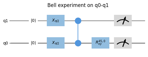
Creates a circuit diagram visualization of a schedule using matplotlib. Each gate, pulse, measurement, and operation are plotted in the order of execution, but the exact timing is not visible here.

Parameters:

• schedule – the schedule to render.

• figsize – matplotlib figsize.

• ax – Axis handle to use for plotting.

Returns:

• fig – matplotlib figure object.

• ax – matplotlib axis object.

Example

from quantify_scheduler import Schedule
from quantify_scheduler.operations.gate_library import Reset, X90, CZ, Rxy, Measure
from quantify_scheduler.visualization.circuit_diagram import circuit_diagram_matplotlib

sched = Schedule(f"Bell experiment on q0-q1")

sched.add(Reset("q0", "q1"))
sched.add(X90("q0"))
sched.add(X90("q1"), ref_pt="start", rel_time=0)
sched.add(CZ(qC="q0", qT="q1"))
sched.add(Rxy(theta=45, phi=0, qubit="q0") )
sched.add(Measure("q0", acq_index=0))
sched.add(Measure("q1", acq_index=0), ref_pt="start")

circuit_diagram_matplotlib(sched);

Note

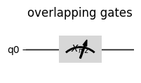
Gates that are started simultaneously on the same qubit will overlap.

from quantify_scheduler import Schedule
from quantify_scheduler.operations.gate_library import X90, Measure

sched = Schedule(f"overlapping gates")

sched.add(X90("q0"))
sched.add(Measure("q0"), ref_pt="start", rel_time=0)
sched.plot_circuit_diagram();

Note

If the pulse’s port address was not found then the pulse will be plotted on the ‘other’ timeline.