User guide
Introduction
A quantify_core experiment typically consists of a data-acquisition loop in
which one or more parameters are set and one or more parameters are measured.
The core of Quantify can be understood by understanding the following concepts:
Code snippets
Bellow we import common utilities used in the examples.
import tempfile
from pathlib import Path

import matplotlib.pyplot as plt
import numpy as np
import xarray as xr
from directory_tree import display_tree
from qcodes import Instrument, ManualParameter, Parameter, validators
from scipy.optimize import minimize_scalar

import quantify_core.data.handling as dh
from quantify_core.analysis import base_analysis as ba
from quantify_core.analysis import cosine_analysis as ca
from quantify_core.measurement import Gettable, MeasurementControl
from quantify_core.utilities.dataset_examples import mk_2d_dataset_v1
from quantify_core.utilities.examples_support import (
    default_datadir,
    mk_cosine_instrument,
)
from quantify_core.utilities.inspect_utils import display_source_code

dh.set_datadir(default_datadir())
meas_ctrl = MeasurementControl("meas_ctrl")
Data will be saved in:
/home/slavoutich/quantify-data
Instruments and Parameters
Parameter
A parameter represents a state variable of the system.
A parameter can be get and/or set able.
Contains metadata such as units and labels.
Commonly implemented using the QCoDeS
Parameterclass.A parameter implemented using the QCoDeS
Parameterclass is a validSettableandGettableand as such can be used directly in an experiment loop in the [Measurement Control]. (see subsequent sections)
Instrument
An Instrument is a container for parameters that typically (but not necessarily) corresponds to a physical piece of hardware.
Instruments provide the following functionality.
Container for parameters.
A standardized interface.
Provide logging of parameters through the
snapshot()method.All instruments inherit from the QCoDeS
Instrumentclass.Are shown by default in the
InstrumentMonitor
Measurement Control
The MeasurementControl (meas_ctrl) is in charge of the data-acquisition loop
and is based on the notion that, in general, an experiment consists of the following
three steps:
Initialize (set) some parameter(s),
Measure (get) some parameter(s),
Store the data.
Quantify provides two helper classes, Settable and Gettable to aid
in these steps, which are explored further in later sections of this article.
MeasurementControl provides the following functionality
Enforce standardization of experiments
Standardized data storage
n-dimensional sweeps
Data acquisition controlled iteratively or in batches
Adaptive sweeps (measurement points are not predetermined at the beginning of an experiment)
Basic example, a 1D iterative measurement loop
Running an experiment is simple! Simply define what parameters to set, and get, and what points to loop over.
In the example below we want to set frequencies on a microwave source and acquire the signal from the pulsar readout module.
meas_ctrl.settables(
    mw_source1.freq
)  # We want to set the frequency of a microwave source
meas_ctrl.setpoints(np.arange(5e9, 5.2e9, 100e3))  # Scan around 5.1 GHz
meas_ctrl.gettables(pulsar_QRM.signal)  # acquire the signal from the pulsar QRM
dset = meas_ctrl.run(name="Frequency sweep")  # run the experiment
Starting iterative measurement...

100% completed | elapsed time:      0s | time left:      0s

100% completed | elapsed time:      0s | time left:      0s
The MeasurementControl can also be used to perform more advanced experiments
such as 2D scans, pulse-sequences where the hardware is in control of the acquisition
loop, or adaptive experiments in which it is not known what data points to acquire in
advance, they are determined dynamically during the experiment.
Take a look at some of the tutorial notebooks for more in-depth examples on
usage and application.
Control Mode
Batched mode can be used to deal with constraints imposed by (hardware) resources or to reduce overhead.
In Iterative mode, the meas_ctrl steps through each setpoint one at a time, processing them one by one.
In Batched mode, the meas_ctrl vectorizes the setpoints such that they are processed in batches. The size of these batches is automatically calculated but usually dependent on resource constraints; you may have a device which can hold 100 samples but you wish to sweep over 2000 points.
Note
The maximum batch size of the settable(s)/gettable(s) should be specified using the
.batch_size attribute. If not specified infinite size is assumed and all setpoint
are passed to the settable(s).
Tip
In Batched mode it is still possible to perform outer iterative sweeps with an inner
batched sweep.
This is performed automatically when batched settables (.batched=True) are mixed
with iterative settables (.batched=False). To correctly grid the points in this mode
use MeasurementControl.setpoints_grid().
Control mode is detected automatically based on the .batched attribute of the
settable(s) and gettable(s); this is expanded upon in subsequent sections.
Note
All gettables must have the same value for the .batched attribute.
Only when all gettables have .batched=True, settables are allowed to have mixed
.batched attribute (e.g. settable_A.batched=True, settable_B.batched=False).
Settables and Gettables
Experiments typically involve varying some parameters and reading others.
In Quantify we encapsulate these concepts as the Settable
and Gettable respectively.
As their name implies, a Settable is a parameter you set values to,
and a Gettable is a parameter you get values from.
The interfaces for Settable and Gettable parameters are encapsulated in the
Settable and Gettable helper classes respectively.
We set values to Settables; these values populate an X-axis.
Similarly, we get values from Gettables which populate a Y-axis.
These classes define a set of mandatory and optional attributes the
MeasurementControl recognizes and will use as part of the experiment,
which are expanded up in the API Reference.
For ease of use, we do not require users to inherit from a Gettable/Settable class,
and instead provide contracts in the form of JSON schemas to which these classes
must fit (see Settable and Gettable docs for these schemas).
In addition to using a library which fits these contracts
(such as the Parameter family of classes)
we can define our own Settables and Gettables.
t = ManualParameter("time", label="Time", unit="s")


class WaveGettable:
    """An examples of a gettable."""

    def __init__(self):
        self.unit = "V"
        self.label = "Amplitude"
        self.name = "sine"

    def get(self):
        """Return the gettable value."""
        return np.sin(t() / np.pi)

    def prepare(self) -> None:
        """Optional methods to prepare can be left undefined."""
        print("Preparing the WaveGettable for acquisition.")

    def finish(self) -> None:
        """Optional methods to finish can be left undefined."""
        print("Finishing WaveGettable to wrap up the experiment.")


# verify compliance with the Gettable format
wave_gettable = WaveGettable()
Gettable(wave_gettable)
<__main__.WaveGettable at 0x7f41481aacd0>
Note: “Grouped” gettable(s) are also allowed.
Below we create a Gettable which returns two distinct quantities at once:
t = ManualParameter(
    "time",
    label="Time",
    unit="s",
    vals=validators.Numbers(),  # accepts a single number, e.g. a float or integer
)


class DualWave1D:
    """Example of a "dual" gettable."""

    def __init__(self):
        self.unit = ["V", "V"]
        self.label = ["Sine Amplitude", "Cosine Amplitude"]
        self.name = ["sin", "cos"]

    def get(self):
        """Return the value of the gettable."""
        return np.array([np.sin(t() / np.pi), np.cos(t() / np.pi)])

    # N.B. the optional prepare and finish methods are omitted in this Gettable.


# verify compliance with the Gettable format
wave_gettable = DualWave1D()
Gettable(wave_gettable)
<__main__.DualWave1D at 0x7f41481aa310>
Depending on which Control Mode the MeasurementControl is running in,
the interfaces for Settables (their input interface) and Gettables
(their output interface) are slightly different.
Note
It is also possible for batched Gettables return an array with length less than then the length of the setpoints, and similarly for the input of the Settables. This is often the case when working with resource constrained devices, for example if you have n setpoints but your device can load only less than n datapoints into memory. In this scenario, the meas_ctrl tracks how many datapoints were actually processed, automatically adjusting the size of the next batch.
Example
time = ManualParameter(
    name="time",
    label="Time",
    unit="s",
    vals=validators.Arrays(),  # accepts an array of values
)
signal = Parameter(
    name="sig_a", label="Signal", unit="V", get_cmd=lambda: np.cos(time())
)

time.batched = True
time.batch_size = 5
signal.batched = True
signal.batch_size = 10

meas_ctrl.settables(time)
meas_ctrl.gettables(signal)
meas_ctrl.setpoints(np.linspace(0, 7, 23))
dset = meas_ctrl.run("my experiment")
dset_grid = dh.to_gridded_dataset(dset)

dset_grid.y0.plot()
Starting batched measurement...
Iterative settable(s) [outer loop(s)]:
	 --- (None) ---
Batched settable(s):
	 time
Batch size limit: 5


100% completed | elapsed time:      0s | time left:      0s  last batch size:      3

100% completed | elapsed time:      0s | time left:      0s  last batch size:      3
[<matplotlib.lines.Line2D at 0x7f410f693730>]
.batched and .batch_size
The Gettable and Settable objects can have a bool property
.batched (defaults to False if not present); and a int property .batch_size.
Setting the .batched property to True enables the batch Control Mode in the
MeasurementControl. In this mode, if present, the .batch_size attribute
is used to determine the maximum size of a batch of setpoints.
Heterogeneous batch size and effective batch size
The minimum .batch_size among all settables and gettables will determine the
(maximum) size of a batch.
During execution of a measurement the size of a batch will be reduced if necessary
to comply to the setpoints grid and/or total number of setpoints.
.prepare() and .finish()
Optionally the .prepare() and .finish() can be added.
These methods can be used to setup and teardown work.
For example, arming a piece of hardware with data and then closing a connection upon
completion.
The .finish() runs once at the end of an experiment.
For settables, .prepare() runs once before the start of a measurement.
For batched gettables, .prepare() runs before the measurement of each batch.
For iterative gettables, the .prepare() runs before each loop counting towards
soft-averages [controlled by meas_ctrl.soft_avg() which resets to 1
at the end of each experiment].
Data storage
Along with the produced dataset, every Parameter
attached to QCoDeS Instrument in an experiment run through
the MeasurementControl of Quantify is stored in the [snapshot].
This is intended to aid with reproducibility, as settings from a past experiment can
easily be reloaded [see load_settings_onto_instrument()].
Data Directory
The top level directory in the file system where output is saved to.
This directory can be controlled using the get_datadir()
and set_datadir() functions.
We recommend to change the default directory when starting the python kernel
(after importing Quantify) and to settle for a single common data directory
for all notebooks/experiments within your measurement setup/PC
(e.g., D:\\quantify-data).
Quantify provides utilities to find/search and extract data, which expects all your experiment containers to be located within the same directory (under the corresponding date subdirectory).
Within the data directory experiments are first grouped by date -
all experiments which take place on a certain date will be saved together in a
subdirectory in the form YYYYmmDD.
Experiment Container
Individual experiments are saved to their own subdirectories (of the Data Directory)
named based on the TUID and the
<experiment name (if any)>.
Note
TUID: A Time-based Unique ID is of the form
YYYYmmDD-HHMMSS-sss-<random 6 character string> and these subdirectories’
names take the form
YYYYmmDD-HHMMSS-sss-<random 6 character string><-experiment name (if any)>.
These subdirectories are termed ‘Experiment Containers’, typical output being the Dataset in hdf5 format and a JSON format file describing Parameters, Instruments and such.
Furthermore, additional analysis such as fits can also be written to this directory, storing all data in one location.
An experiment container within a data directory with the name "quantify-data"
thus will look similar to:
quantify-data/
├── 20210301/
├── 20210428/
└── 20230926/
    └── 20230926-194517-639-5bd4b0-my experiment/
        ├── analysis_BasicAnalysis/
        │   ├── dataset_processed.hdf5
        │   ├── figs_mpl/
        │   │   ├── Line plot x0-y0.png
        │   │   ├── Line plot x0-y0.svg
        │   │   ├── Line plot x1-y0.png
        │   │   └── Line plot x1-y0.svg
        │   └── quantities_of_interest.json
        └── dataset.hdf5
Dataset
The Dataset is implemented with a specific convention using the
xarray.Dataset class.
Quantify arranges data along two types of axes: X and Y.
In each dataset there will be n X-type axes and m Y-type axes.
For example, the dataset produced in an experiment where we sweep 2 parameters (settables)
and measure 3 other parameters (all 3 returned by a Gettable),
we will have n = 2 and m = 3.
Each X axis represents a dimension of the setpoints provided.
The Y axes represent the output of the Gettable.
Each axis type are numbered ascending from 0
(e.g. x0, x1, y0, y1, y2),
and each stores information described by the Settable and Gettable
classes, such as titles and units.
The Dataset object also stores some further metadata,
such as the TUID of the experiment which it was
generated from.
For example, consider an experiment varying time and amplitude against a Cosine function. The resulting dataset will look similar to the following:
# plot the columns of the dataset
_, axs = plt.subplots(3, 1, sharex=True)
xr.plot.line(quantify_dataset.x0[:54], label="x0", ax=axs[0], marker=".")
xr.plot.line(quantify_dataset.x1[:54], label="x1", ax=axs[1], color="C1", marker=".")
xr.plot.line(quantify_dataset.y0[:54], label="y0", ax=axs[2], color="C2", marker=".")
tuple(ax.legend() for ax in axs)
# return the dataset
quantify_dataset
<xarray.Dataset>
Dimensions:  (dim_0: 1000)
Coordinates:
    x0       (dim_0) float64 -1.0 -0.7778 -0.5556 -0.3333 ... 0.5556 0.7778 1.0
    x1       (dim_0) float64 0.0 0.0 0.0 0.0 0.0 ... 10.0 10.0 10.0 10.0 10.0
Dimensions without coordinates: dim_0
Data variables:
    y0       (dim_0) float64 -1.0 -0.7778 -0.5556 ... -0.4662 -0.6526 -0.8391
Attributes:
    tuid:                      20230926-194517-639-5bd4b0
    name:                      my experiment
    grid_2d:                   True
    grid_2d_uniformly_spaced:  True
    xlen:                      10
    ylen:                      100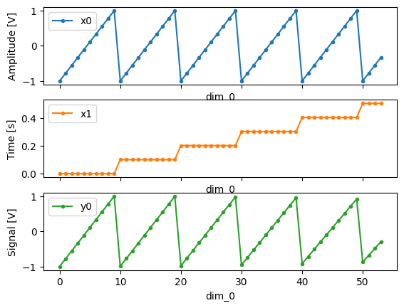
Associating dimensions to coordinates
To support both gridded and non-gridded data, we use Xarray
using only Data Variables and Coordinates with a single Dimension
(corresponding to the order of the setpoints).
This is necessary as in the non-gridded case the dataset will be a perfect sparse array, usability of which is cumbersome. A prominent example of non-gridded use-cases can be found Tutorial 4. Adaptive Measurements.
To allow for some of Xarray’s more advanced functionality,
such as the in-built graphing or query system we provide a dataset conversion utility
to_gridded_dataset().
This function reshapes the data and associates dimensions to the dataset
[which can also be used for 1D datasets].
gridded_dset = dh.to_gridded_dataset(quantify_dataset)
gridded_dset.y0.plot()
gridded_dset
<xarray.Dataset>
Dimensions:  (x0: 10, x1: 100)
Coordinates:
  * x0       (x0) float64 -1.0 -0.7778 -0.5556 -0.3333 ... 0.5556 0.7778 1.0
  * x1       (x1) float64 0.0 0.101 0.202 0.303 0.404 ... 9.697 9.798 9.899 10.0
Data variables:
    y0       (x0, x1) float64 -1.0 -0.9949 -0.9797 ... -0.9312 -0.8897 -0.8391
Attributes:
    tuid:                      20230926-194517-639-5bd4b0
    name:                      my experiment
    grid_2d:                   False
    grid_2d_uniformly_spaced:  True
    xlen:                      10
    ylen:                      100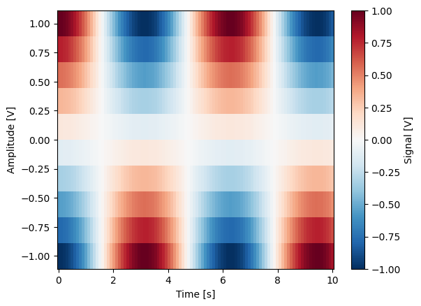
Snapshot
The configuration for each QCoDeS Instrument
used in this experiment.
This information is automatically collected for all Instruments in use.
It is useful for quickly reconstructing a complex set-up or verifying that
Parameter objects are as expected.
Analysis
To aid with data analysis, quantify comes with an analysis module
containing a base data-analysis class
(BaseAnalysis)
that is intended to serve as a template for analysis scripts
and several standard analyses such as
the BasicAnalysis,
the Basic2DAnalysis
and the ResonatorSpectroscopyAnalysis.
The idea behind the analysis class is that most analyses follow a common structure consisting of steps such as data extraction, data processing, fitting to some model, creating figures, and saving the analysis results.
To showcase the analysis usage we generates a dataset that we would like to analyze.
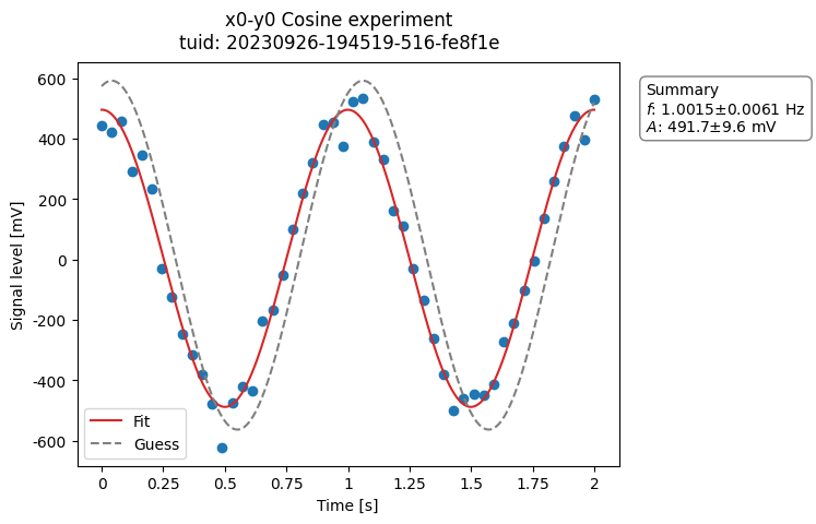
Generate a dataset labeled “Cosine experiment”
display_source_code(mk_cosine_instrument)
def mk_cosine_instrument() -> Instrument:
    """A container of parameters (mock instrument) providing a cosine model."""

    instr = Instrument("ParameterHolder")

    # ManualParameter's is a handy class that preserves the QCoDeS' Parameter
    # structure without necessarily having a connection to the physical world
    instr.add_parameter(
        "amp",
        initial_value=0.5,
        unit="V",
        label="Amplitude",
        parameter_class=ManualParameter,
    )
    instr.add_parameter(
        "freq",
        initial_value=1,
        unit="Hz",
        label="Frequency",
        parameter_class=ManualParameter,
    )
    instr.add_parameter(
        "t", initial_value=1, unit="s", label="Time", parameter_class=ManualParameter
    )
    instr.add_parameter(
        "phi",
        initial_value=0,
        unit="Rad",
        label="Phase",
        parameter_class=ManualParameter,
    )
    instr.add_parameter(
        "noise_level",
        initial_value=0.05,
        unit="V",
        label="Noise level",
        parameter_class=ManualParameter,
    )
    instr.add_parameter(
        "acq_delay", initial_value=0.02, unit="s", parameter_class=ManualParameter
    )

    def cosine_model():
        sleep(instr.acq_delay())  # simulates the acquisition delay of an instrument
        return (
            cos_func(instr.t(), instr.freq(), instr.amp(), phase=instr.phi(), offset=0)
            + np.random.randn() * instr.noise_level()
        )

    # Wrap our function in a Parameter to be able to associate metadata to it, e.g. unit
    instr.add_parameter(
        name="sig", label="Signal level", unit="V", get_cmd=cosine_model
    )

    return instr
pars = mk_cosine_instrument()
meas_ctrl.settables(pars.t)
meas_ctrl.setpoints(np.linspace(0, 2, 50))
meas_ctrl.gettables(pars.sig)
dataset = meas_ctrl.run("Cosine experiment")
dataset
Starting iterative measurement...

  2% completed | elapsed time:      0s | time left:      1s
  2% completed | elapsed time:      0s | time left:      1s
 52% completed | elapsed time:      0s | time left:      0s
 52% completed | elapsed time:      0s | time left:      0s
100% completed | elapsed time:      1s | time left:      0s

100% completed | elapsed time:      1s | time left:      0s
<xarray.Dataset>
Dimensions:  (dim_0: 50)
Coordinates:
    x0       (dim_0) float64 0.0 0.04082 0.08163 0.1224 ... 1.918 1.959 2.0
Dimensions without coordinates: dim_0
Data variables:
    y0       (dim_0) float64 0.4427 0.4202 0.4573 0.2919 ... 0.4737 0.3959 0.528
Attributes:
    tuid:                             20230926-194519-516-fe8f1e
    name:                             Cosine experiment
    grid_2d:                          False
    grid_2d_uniformly_spaced:         False
1d_2_settables_uniformly_spaced: FalseUsing an analysis class
Running an analysis is very simple:
a_obj = ca.CosineAnalysis(label="Cosine experiment")
a_obj.run()  # execute the analysis.
a_obj.display_figs_mpl()  # displays the figures created in previous step.
The analysis was executed against the last dataset that has the label
"Cosine experiment" in the filename.
After the analysis the experiment container will look similar to the following:
experiment_container_path = dh.locate_experiment_container(tuid=dataset.tuid)
print(display_tree(experiment_container_path, string_rep=True), end="")
20230926-194519-516-fe8f1e-Cosine experiment/
├── analysis_CosineAnalysis/
│   ├── dataset_processed.hdf5
│   ├── figs_mpl/
│   │   ├── cos_fit.png
│   │   └── cos_fit.svg
│   ├── fit_results/
│   │   └── cosine.txt
│   └── quantities_of_interest.json
├── dataset.hdf5
└── snapshot.json
The analysis object contains several useful methods and attributes such as the
quantities_of_interest, intended to store relevant quantities extracted
during analysis, and the processed dataset.
# for example, the fitted frequency and amplitude are stored
freq = a_obj.quantities_of_interest["frequency"]
amp = a_obj.quantities_of_interest["amplitude"]
print(f"frequency {freq}")
print(f"amplitude {amp}")
frequency 1.001+/-0.006
amplitude 0.492+/-0.010
The use of these methods and attributes is described in more detail in Tutorial 3. Building custom analyses - the data analysis framework.
Creating a custom analysis class
The analysis steps and their order of execution is determined by the
analysis_steps attribute
as an Enum (AnalysisSteps).
The corresponding steps are implemented as methods of the analysis class.
An analysis class inheriting from the abstract-base-class
(BaseAnalysis)
will only have to implement those methods that are unique to the custom analysis.
Additionally, if required, a customized analysis flow can be specified by assigning it
to the analysis_steps attribute.
The simplest example of an analysis class is the
BasicAnalysis
that only implements the
create_figures() method
and relies on the base class for data extraction and saving of the figures.
Take a look at the source code (also available in the API reference):
BasicAnalysis source code
display_source_code(ba.BasicAnalysis)
class BasicAnalysis(BaseAnalysis):
    """
    A basic analysis that extracts the data from the latest file matching the label
    and plots and stores the data in the experiment container.
    """

    def create_figures(self):
        """
        Creates a line plot x vs y for every data variable yi and coordinate xi in the
        dataset.
        """

        # NB we do not use `to_gridded_dataset` because that can potentially drop
        # repeated measurement of the same x0_i setpoint (e.g., AllXY experiment)
        dataset = self.dataset
        # for compatibility with older datasets
        # in case "x0" is not a coordinate we use "dim_0"
        coords = list(dataset.coords)
        dims = list(dataset.dims)
        plot_against = coords if coords else (dims if dims else [None])
        for idx, xi in enumerate(plot_against):
            for yi, yvals in dataset.data_vars.items():
                # for compatibility with older datasets, do not plot "x0" vs "x0"
                if yi.startswith("y"):
                    fig, ax = plt.subplots()

                    fig_id = f"Line plot x{idx}-{yi}"

                    yvals.plot.line(ax=ax, x=xi, marker=".")

                    adjust_axeslabels_SI(ax)

                    qpl.set_suptitle_from_dataset(fig, self.dataset, f"x{idx}-{yi}")

                    # add the figure and axis to the dicts for saving
                    self.figs_mpl[fig_id] = fig
                    self.axs_mpl[fig_id] = ax
A slightly more complex use case is the
ResonatorSpectroscopyAnalysis
that implements
process_data()
to cast the data to a complex-valued array,
run_fitting()
where a fit is performed using a model
(from the quantify_core.analysis.fitting_models library), and
create_figures()
where the data and the fitted curve are plotted together.
Creating a custom analysis for a particular type of dataset is showcased in the Tutorial 3. Building custom analyses - the data analysis framework. There you will also learn some other capabilities of the analysis and practical productivity tips.
Examples: Settables and Gettables
Below we give several examples of experiment using Settables and Gettables in different control modes.
Iterative control mode
Single-float-valued settable(s) and gettable(s)
Each settable accepts a single float value.
Gettables return a single float value.
1D
time = ManualParameter(
    name="time", label="Time", unit="s", vals=validators.Numbers(), initial_value=1
)
signal = Parameter(
    name="sig_a", label="Signal", unit="V", get_cmd=lambda: np.cos(time())
)

meas_ctrl.settables(time)
meas_ctrl.gettables(signal)
meas_ctrl.setpoints(np.linspace(0, 7, 20))
dset = meas_ctrl.run("my experiment")
dset_grid = dh.to_gridded_dataset(dset)

dset_grid.y0.plot(marker="o")
dset_grid
Starting iterative measurement...

  5% completed | elapsed time:      0s | time left:      0s
  5% completed | elapsed time:      0s | time left:      0s
100% completed | elapsed time:      0s | time left:      0s

100% completed | elapsed time:      0s | time left:      0s
<xarray.Dataset>
Dimensions:  (x0: 20)
Coordinates:
  * x0       (x0) float64 0.0 0.3684 0.7368 1.105 ... 5.895 6.263 6.632 7.0
Data variables:
    y0       (x0) float64 1.0 0.9329 0.7406 0.4489 ... 0.9998 0.9399 0.7539
Attributes:
    tuid:                             20230926-194521-660-4220d2
    name:                             my experiment
    grid_2d:                          False
    grid_2d_uniformly_spaced:         False
    1d_2_settables_uniformly_spaced:  False
2D
time_a = ManualParameter(
name="time_a", label="Time A", unit="s", vals=validators.Numbers(), initial_value=1
)
time_b = ManualParameter(
name="time_b", label="Time B", unit="s", vals=validators.Numbers(), initial_value=1
)
signal = Parameter(
name="sig_a",
label="Signal A",
unit="V",
get_cmd=lambda: np.exp(time_a()) + 0.5 * np.exp(time_b()),
)

meas_ctrl.settables([time_a, time_b])
meas_ctrl.gettables(signal)
meas_ctrl.setpoints_grid([np.linspace(0, 5, 10), np.linspace(5, 0, 12)])
dset = meas_ctrl.run("my experiment")
dset_grid = dh.to_gridded_dataset(dset)

dset_grid.y0.plot(cmap="viridis")
dset_grid
Starting iterative measurement...

100% completed | elapsed time:      0s | time left:      0s

100% completed | elapsed time:      0s | time left:      0s
<xarray.Dataset>
Dimensions:  (x0: 10, x1: 12)
Coordinates:
  * x0       (x0) float64 0.0 0.5556 1.111 1.667 2.222 ... 3.333 3.889 4.444 5.0
  * x1       (x1) float64 0.0 0.4545 0.9091 1.364 ... 3.636 4.091 4.545 5.0
Data variables:
    y0       (x0, x1) float64 1.5 1.788 2.241 2.955 ... 167.4 178.3 195.5 222.6
Attributes:
    tuid:                             20230926-194521-916-a44111
    name:                             my experiment
    grid_2d:                          False
    grid_2d_uniformly_spaced:         True
    1d_2_settables_uniformly_spaced:  False
    xlen:                             10
    ylen:                             12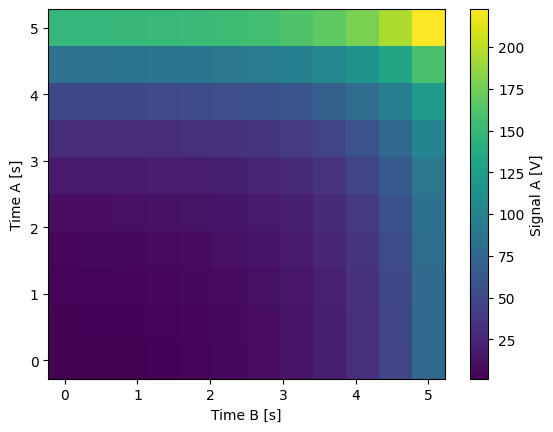
ND
For more dimensions you only need to pass more settables and the corresponding setpoints.
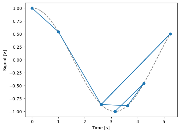
1D adaptive
time = ManualParameter(
    name="time", label="Time", unit="s", vals=validators.Numbers(), initial_value=1
)
signal = Parameter(
    name="sig_a", label="Signal", unit="V", get_cmd=lambda: np.cos(time())
)
meas_ctrl.settables(time)
meas_ctrl.gettables(signal)
dset = meas_ctrl.run_adaptive("1D minimizer", {"adaptive_function": minimize_scalar})

dset_ad = dh.to_gridded_dataset(dset)
# add a grey cosine for reference
x = np.linspace(np.min(dset_ad["x0"]), np.max(dset_ad["x0"]), 101)
y = np.cos(x)
plt.plot(x, y, c="grey", ls="--")
_ = dset_ad.y0.plot(marker="o")
Running adaptively...
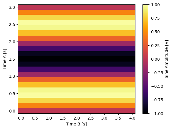
Single-float-valued settable(s) with multiple float-valued gettable(s)
Each settable accepts a single float value.
Gettables return a 1D array of floats, with each element corresponding to a different Y dimension.
We exemplify a 2D case, however there is no limitation on the number of settables.
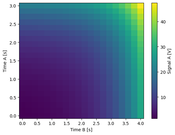
2D
time_a = ManualParameter(
name="time_a", label="Time A", unit="s", vals=validators.Numbers(), initial_value=1
)
time_b = ManualParameter(
name="time_b", label="Time B", unit="s", vals=validators.Numbers(), initial_value=1
)
signal = Parameter(
name="sig_a",
label="Signal A",
unit="V",
get_cmd=lambda: np.exp(time_a()) + 0.5 * np.exp(time_b()),
)
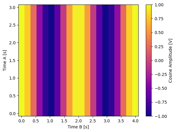
class DualWave2D:
"""A "dual" gettable example that depends on two settables."""
def __init__(self):
self.unit = ["V", "V"]
self.label = ["Sine Amplitude", "Cosine Amplitude"]
self.name = ["sin", "cos"]
def get(self):
"""Returns the value of the gettable."""
return np.array([np.sin(time_a() * np.pi), np.cos(time_b() * np.pi)])
dual_wave = DualWave2D()
meas_ctrl.settables([time_a, time_b])
meas_ctrl.gettables([signal, dual_wave])
meas_ctrl.setpoints_grid([np.linspace(0, 3, 21), np.linspace(4, 0, 20)])
dset = meas_ctrl.run("my experiment")
dset_grid = dh.to_gridded_dataset(dset)
for yi, cmap in zip(("y0", "y1", "y2"), ("viridis", "inferno", "plasma")):
dset_grid[yi].plot(cmap=cmap)
plt.show()
dset_grid
Starting iterative measurement...

100% completed | elapsed time:      0s | time left:      0s

100% completed | elapsed time:      0s | time left:      0s
<xarray.Dataset>
Dimensions:  (x0: 21, x1: 20)
Coordinates:
  * x0       (x0) float64 0.0 0.15 0.3 0.45 0.6 0.75 ... 2.4 2.55 2.7 2.85 3.0
  * x1       (x1) float64 0.0 0.2105 0.4211 0.6316 ... 3.368 3.579 3.789 4.0
Data variables:
    y0       (x0, x1) float64 1.5 1.617 1.762 1.94 ... 34.6 38.0 42.2 47.38
    y1       (x0, x1) float64 0.0 0.0 0.0 0.0 ... 3.674e-16 3.674e-16 3.674e-16
    y2       (x0, x1) float64 1.0 0.7891 0.2455 -0.4017 ... 0.2455 0.7891 1.0
Attributes:
    tuid:                             20230926-194522-396-00bd89
    name:                             my experiment
    grid_2d:                          False
    grid_2d_uniformly_spaced:         True
    1d_2_settables_uniformly_spaced:  True
    xlen:                             21
ylen: 20Batched control mode
Float-valued array settable(s) and gettable(s)
Gettables return a 1D array of float values with each element corresponding to a datapoint in a single Y dimension.
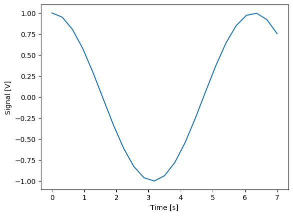
1D
Each settable accepts a 1D array of float values corresponding to all setpoints for a single X dimension.
time = ManualParameter(
    name="time",
    label="Time",
    unit="s",
    vals=validators.Arrays(),
    initial_value=np.array([1, 2, 3]),
)
signal = Parameter(
    name="sig_a", label="Signal", unit="V", get_cmd=lambda: np.cos(time())
)

time.batched = True
signal.batched = True

meas_ctrl.settables(time)
meas_ctrl.gettables(signal)
meas_ctrl.setpoints(np.linspace(0, 7, 20))
dset = meas_ctrl.run("my experiment")
dset_grid = dh.to_gridded_dataset(dset)

dset_grid.y0.plot(marker="o")
print(f"\nNOTE: The gettable returns an array:\n\n{signal.get()}")
dset_grid
Starting batched measurement...
Iterative settable(s) [outer loop(s)]:
	 --- (None) ---
Batched settable(s):
	 time
Batch size limit: 20


100% completed | elapsed time:      0s | time left:      0s  last batch size:     20

100% completed | elapsed time:      0s | time left:      0s  last batch size:     20
NOTE: The gettable returns an array:

[ 1.          0.93289715  0.7405942   0.4488993   0.09695955 -0.26799272
 -0.59697884 -0.84584701 -0.98119769 -0.98486606 -0.8563598  -0.61292518
 -0.28723252  0.07700839  0.43091433  0.72698911  0.92549782  0.99979946
  0.93992232  0.75390225]
<xarray.Dataset>
Dimensions:  (x0: 20)
Coordinates:
  * x0       (x0) float64 0.0 0.3684 0.7368 1.105 ... 5.895 6.263 6.632 7.0
Data variables:
    y0       (x0) float64 1.0 0.9329 0.7406 0.4489 ... 0.9998 0.9399 0.7539
Attributes:
    tuid:                             20230926-194523-091-e64930
    name:                             my experiment
    grid_2d:                          False
    grid_2d_uniformly_spaced:         False
    1d_2_settables_uniformly_spaced:  False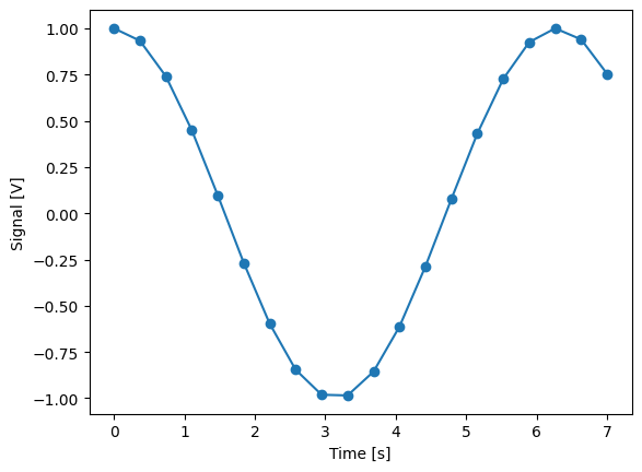
2D (1D batch with iterative outer loop)
One settable (at least) accepts a 1D array of float values corresponding to all setpoints for the corresponding X dimension.
One settable (at least) accepts a float value corresponding to its X dimension. The meas_ctrl will set the value of each of these iterative settables before each batch.
time_a = ManualParameter(
    name="time_a", label="Time A", unit="s", vals=validators.Numbers(), initial_value=1
)
time_b = ManualParameter(
    name="time_b",
    label="Time B",
    unit="s",
    vals=validators.Arrays(),
    initial_value=np.array([1, 2, 3]),
)
signal = Parameter(
    name="sig_a",
    label="Signal A",
    unit="V",
    get_cmd=lambda: np.exp(time_a()) + 0.5 * np.exp(time_b()),
)

time_b.batched = True
time_b.batch_size = 12
signal.batched = True

meas_ctrl.settables([time_a, time_b])
meas_ctrl.gettables(signal)
# `setpoints_grid` will take into account the `.batched` attribute
meas_ctrl.setpoints_grid([np.linspace(0, 5, 10), np.linspace(4, 0, time_b.batch_size)])
dset = meas_ctrl.run("my experiment")
dset_grid = dh.to_gridded_dataset(dset)

dset_grid.y0.plot(cmap="viridis")
dset_grid
Starting batched measurement...
Iterative settable(s) [outer loop(s)]:
	 time_a
Batched settable(s):
	 time_b
Batch size limit: 12


100% completed | elapsed time:      0s | time left:      0s  last batch size:     12

100% completed | elapsed time:      0s | time left:      0s  last batch size:     12
<xarray.Dataset>
Dimensions:  (x0: 10, x1: 12)
Coordinates:
  * x0       (x0) float64 0.0 0.5556 1.111 1.667 2.222 ... 3.333 3.889 4.444 5.0
  * x1       (x1) float64 0.0 0.3636 0.7273 1.091 ... 2.909 3.273 3.636 4.0
Data variables:
    y0       (x0, x1) float64 1.5 1.719 2.035 2.488 ... 157.6 161.6 167.4 175.7
Attributes:
    tuid:                             20230926-194523-347-529783
    name:                             my experiment
    grid_2d:                          False
    grid_2d_uniformly_spaced:         True
    1d_2_settables_uniformly_spaced:  False
    xlen:                             10
    ylen:                             12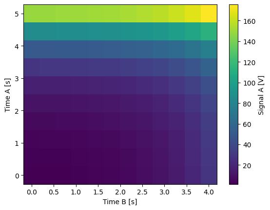
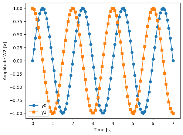
Float-valued array settable(s) with multi-return float-valued array gettable(s)
Each settable accepts a 1D array of float values corresponding to all setpoints for a single X dimension.
Gettables return a 2D array of float values with each row representing a different Y dimension, i.e. each column is a datapoint corresponding to each setpoint.
1D
time = ManualParameter(
    name="time",
    label="Time",
    unit="s",
    vals=validators.Arrays(),
    initial_value=np.array([1, 2, 3]),
)


class DualWaveBatched:
    """A "dual" batched gettable example."""

    def __init__(self):
        self.unit = ["V", "V"]
        self.label = ["Amplitude W1", "Amplitude W2"]
        self.name = ["sine", "cosine"]
        self.batched = True
        self.batch_size = 100

    def get(self):
        """Returns the value of the gettable."""
        return np.array([np.sin(time() * np.pi), np.cos(time() * np.pi)])


time.batched = True
dual_wave = DualWaveBatched()

meas_ctrl.settables(time)
meas_ctrl.gettables(dual_wave)
meas_ctrl.setpoints(np.linspace(0, 7, 100))
dset = meas_ctrl.run("my experiment")
dset_grid = dh.to_gridded_dataset(dset)

_, ax = plt.subplots()
dset_grid.y0.plot(marker="o", label="y0", ax=ax)
dset_grid.y1.plot(marker="s", label="y1", ax=ax)
_ = ax.legend()
Starting batched measurement...
Iterative settable(s) [outer loop(s)]:
	 --- (None) ---
Batched settable(s):
	 time
Batch size limit: 100


100% completed | elapsed time:      0s | time left:      0s  last batch size:    100

100% completed | elapsed time:      0s | time left:      0s  last batch size:    100