Hardware backends

The compiler for a hardware backend for Quantify takes a Schedule defined on the Quantum-device layer and a HardwareCompilationConfig. The InstrumentCoordinatorComponent for the hardware runs the operations within the schedule and can return the acquired data via the InstrumentCoordinator method retrieve_acquisition(). To that end, it generally consists of the following components:

1. CompilationNodes that generate the compiled Schedule from the device-level Schedule and a HardwareCompilationConfig. This compiled Schedule generally consists of (1) the hardware level instructions that should be executed and (2) instrument settings that should be applied on the hardware.

2. A backend-specific HardwareCompilationConfig that contains the information that is used to compile from the quantum-device layer to the control-hardware layer (see Compilation). This generally consists of:

   • A HardwareDescription (e.g., the available channels, IP addresses, etc.).

   • The Connectivity between the quantum-device ports and the control-hardware ports.

   • The HardwareOptions that includes the specific settings that are supported by the backend (e.g., the gain on an output port).

   • A list of SimpleNodeConfigs, which specifies the CompilationNodes that should be executed to compile the Schedule to the hardware-specific instructions.

3. InstrumentCoordinatorComponents that send compiled instructions to the instruments, retrieve data, and convert the acquired data into a standardized, backend independent dataset (see Acquisition protocols).

Architecture overview

The interfaces between Quantify and a hardware backend are illustrated in the following diagram:

        graph TD;
    user[User]

    subgraph Quantify
        ScheduleGettable
        QuantumDevice
        QuantifyCompiler
        InstrumentCoordinator
    
        QuantumDevice -->|CompilationConfig| ScheduleGettable
        ScheduleGettable -->|Schedule\n CompilationConfig| QuantifyCompiler
        InstrumentCoordinator -->|Raw Dataset| ScheduleGettable
        QuantifyCompiler -->|CompiledSchedule| ScheduleGettable
        ScheduleGettable -->|CompiledSchedule| InstrumentCoordinator
    end

    subgraph QuantifyBackend
        InstrumentCoordinatorComponent
        CompilationModule[Compilation Module] -->|CompilationNodes| HardwareCompilationConfig
        HardwareCompilationConfig
    end

    subgraph Hardware
        drivers[Hardware-specific drivers]
        instruments[Physical instruments]
    end

    user -->|Schedule| ScheduleGettable
    user -->|Device Description, Hardware Description,\n Connectivity, Hardware Options| QuantumDevice
    ScheduleGettable -->|Processed Dataset| user

    InstrumentCoordinatorComponent -->|Partial Raw Dataset| InstrumentCoordinator
    QuantumDevice -->|Hardware Description\n Connectivity\n Hardware Options| HardwareCompilationConfig
    HardwareCompilationConfig -->|Validated HardwareCompilationConfig| QuantumDevice
    
    InstrumentCoordinator -->|Compiled Instructions| InstrumentCoordinatorComponent

    InstrumentCoordinatorComponent -->|Compiled Instructions| drivers
    drivers -->|Data points| InstrumentCoordinatorComponent

    drivers <--> instruments
    

Experiment flow

See also

This diagram is similar to the the one in the Experiment flow section in the User Guide, but provides more details on the interfaces between the objects.

        sequenceDiagram
    participant SG as ScheduleGettable
    participant QuantumDevice
    participant QuantifyCompiler
    participant IC as InstrumentCoordinator
    SG->>+QuantumDevice: generate_compilation_config()
    QuantumDevice-->>-SG: CompilationConfig
    SG->>+QuantifyCompiler: compile(Schedule, CompilationConfig)
    QuantifyCompiler-->>-SG: CompiledSchedule
    SG->>+IC: prepare(CompiledSchedule)
    SG->>IC: start()
    SG->>IC: retrieve_acquisition()
    IC-->>-SG: RawDataset	
    

Fig. 6 Diagram of the experiment flow in Quantify. Dotted lines represent the output and the non-dotted lines represent the input.

In the above diagram several methods are called. The get() method of the ScheduleGettable executes the sequence and returns the data from the acquisitions in the Schedule. The generate_compilation_config() method of the QuantumDevice generates a CompilationConfig that is used to compile the Schedule within the ScheduleGettable. The compile() method of the QuantifyCompiler compiles the Schedule to the hardware-specific instructions. The prepare(), start(), and retrieve_acquisition() methods of the InstrumentCoordinator are used to prepare the hardware, start the acquisition, and retrieve the acquired data, respectively.

Developing a new backend

To develop a new backend, the following approach is advised:

1. Implement a custom Gettable that takes a set of instructions in the form that the hardware can directly execute. The compiled schedule that the backend should return once developed should therefore be the same as the instructions that this Gettable accepts. This enables testing of the InstrumentCoordinatorComponents without having to worry about the compilation of the Schedule to the hardware.

2. Implement InstrumentCoordinatorComponents for each of the instruments (starting with the instrument with the acquisition channel to enable testing).

3. Implement CompilationNodes to generate hardware instructions from a Schedule and a CompilationConfig.

4. Integrate the (previously developed + tested) QuantifyCompiler and InstrumentCoordinatorComponents with the ScheduleGettable.

5. Optionally test the ScheduleGettable with the MeasurementControl.

Mock device

To illustrate how to do this, let’s consider a basic example of an interface with a mock hardware device for which we would like to create a corresponding Quantify hardware backend. Our mock device resembles a readout module that can play and simultaneously acquire waveforms through the “TRACE” instruction. It is described by the following class:

class MockReadoutModule(name: str, sampling_rate: float = 1000000000.0, gain: float = 1.0)

Mock readout module that just supports “TRACE” instruction.

The device has three methods, execute, upload_waveforms, and upload_instructions, and a property sampling_rate.

In our endeavor to create a backend between Quantify and the mock device we start by creating a mock readout module so we can show its functionality:

import numpy as np
from quantify_scheduler.backends.mock.mock_rom import MockReadoutModule

rom = MockReadoutModule(name="mock_rom")

We first upload two waveforms (defined on a 1 ns grid) to the readout module:

intermodulation_freq = 1e8  # 100 MHz
amplitude = 0.5 # 0.5 V
duration = 1e-7  # 100 ns

time_grid = np.arange(0, duration, 1e-9)
complex_trace = np.exp(2j * np.pi * intermodulation_freq * time_grid)

wfs = {
    "I": complex_trace.real,
    "Q": complex_trace.imag
}
rom.upload_waveforms(wfs)

The mock readout module samples the uploaded waveforms and applies a certain gain to the acquired data. The sampling rate and gain can be set as follows:

rom.sampling_rate = 1.5e9  # 1.5 GSa/s
rom.gain = 2.0

The mock readout module takes a list of strings as instructions input:

rom.upload_instructions(["TRACE_input0_0"])

We can now execute the instructions on the readout module:

rom.execute()

The data that is returned by our mock readout module is a dictionary containing the acquired I and Q traces:

import matplotlib.pyplot as plt

data = rom.get_results()
plt.plot(data[0][0])
plt.plot(data[0][1])
plt.show()

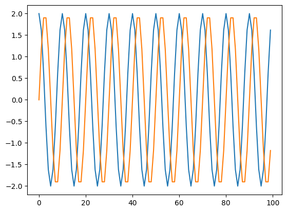
The goal is now to implement a backend that can compile and execute a Schedule that consists of a single trace acquisition and returns a Quantify dataset.

1. Implement a custom Gettable

A good first step to integrating this mock readout module with Quantify is to implement a custom Gettable that takes a set of instructions and waveforms that can be readily executed on the hardware. This Gettable can then be used to retrieve the executed waveforms from the hardware. This enables testing of the InstrumentCoordinatorComponents without having to worry about the compilation of the Schedule to the hardware.

class MockROMGettable(mock_rom: MockReadoutModule, waveforms: dict[str, quantify_scheduler.structure.types.NDArray], instructions: list[str], sampling_rate: float = 1000000000.0, gain: float = 1.0)

Mock readout module gettable.

We check that this works as expected:

from quantify_scheduler.backends.mock.mock_rom import MockROMGettable

mock_rom_gettable = MockROMGettable(mock_rom=rom, waveforms=wfs, instructions=["TRACE_input0_0"], sampling_rate=1.5e9, gain=2.0)
data = mock_rom_gettable.get()
plt.plot(data[0][0])
plt.plot(data[0][1])
plt.show()

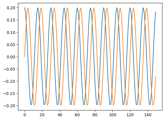
From the plot, we observe that the waveforms are the same as what was sent into the MockReadoutModule.

2. Acquisition mappings

With regards to acquisition data, the ultimate role of the backend is to map the acquisition data on the hardware to the returned structured data (xarray.Dataset). This mapping must be generated at compilation time, and then after the experiment is run on the hardware, this mapping is needed to generate the returned structured xarray.Dataset to the user.

The structured acquisition data consists of an xarray.Dataset, which is practically a dictionary where the keys are user given acquisition channel names and the values are the corresponding data to that acquisition channel. The acquisition channel data xarray.DataArray is one dimensional data (assuming no append mode repetitions): each acquired data point has an index (acquisition index), and other user-given coordinates.

As an example, in case of several binned acquisition (multiple acquisition indices), but on the same acquisition channel, a typical data looks like the following for a schedule.

schedule = Schedule("example")
schedule.add(Measure(qubit="q0", acq_channel="ch_0", coords={"freq": 100}))
schedule.add(Measure(qubit="q0", acq_channel="ch_0", coords={"freq": 200}))
schedule.add(Measure(qubit="q0", acq_channel="ch_0", coords={"freq": 300}))

Show code cell source

Hide code cell source

import xarray

xarray.Dataset(
    data_vars=dict(
        ch_0=(["acq_index_ch_0"], [0.0, 0.2, 0.4]),
    ),
    coords=dict(
        freq=(["acq_index_ch_0"], [100, 200, 300]),
        acq_index_ch_0=[0, 1, 2],
    ),
)

<xarray.Dataset> Size: 72B
Dimensions:         (acq_index_ch_0: 3)
Coordinates:
    freq            (acq_index_ch_0) int64 24B 100 200 300
  * acq_index_ch_0  (acq_index_ch_0) int64 24B 0 1 2
Data variables:
    ch_0            (acq_index_ch_0) float64 24B 0.0 0.2 0.4

xarray.Dataset

• Dimensions:
  • acq_index_ch_0: 3
• Coordinates: (2)
  • freq
    (acq_index_ch_0)
    int64
    100 200 300

    array([100, 200, 300])

  • acq_index_ch_0
    (acq_index_ch_0)
    int64
    0 1 2

    array([0, 1, 2])

• Data variables: (1)
  • ch_0
    (acq_index_ch_0)
    float64
    0.0 0.2 0.4

    array([0. , 0.2, 0.4])

• Indexes: (1)
  • acq_index_ch_0
    PandasIndex

    PandasIndex(Index([0, 1, 2], dtype='int64', name='acq_index_ch_0'))

• Attributes: (0)

In case of trace acquisition, there is one acquisition index, and the other dimension is the time for our mock backend.

schedule = Schedule("example")
schedule.add(Measure(qubit="q0", acq_channel="ch_0", acq_protocol="Trace"))

Show code cell source

Hide code cell source

import xarray

xarray.Dataset(
    data_vars=dict(
        ch_0=(["acq_index_ch_0", "time_ch0"], [[2.5, 2.6, 2.7, 2.8, 2.9, 3.0]]),
    ),
    coords=dict(
        time_ch0=[0.0, 0.001, 0.002, 0.003, 0.004, 0.005],
        acq_index_ch_0=[0],
    ),
)

<xarray.Dataset> Size: 104B
Dimensions:         (acq_index_ch_0: 1, time_ch0: 6)
Coordinates:
  * time_ch0        (time_ch0) float64 48B 0.0 0.001 0.002 0.003 0.004 0.005
  * acq_index_ch_0  (acq_index_ch_0) int64 8B 0
Data variables:
    ch_0            (acq_index_ch_0, time_ch0) float64 48B 2.5 2.6 ... 2.9 3.0

xarray.Dataset

• Dimensions:
  • acq_index_ch_0: 1
  • time_ch0: 6
• Coordinates: (2)
  • time_ch0
    (time_ch0)
    float64
    0.0 0.001 0.002 0.003 0.004 0.005

    array([0.   , 0.001, 0.002, 0.003, 0.004, 0.005])

  • acq_index_ch_0
    (acq_index_ch_0)
    int64
    0

    array([0])

• Data variables: (1)
  • ch_0
    (acq_index_ch_0, time_ch0)
    float64
    2.5 2.6 2.7 2.8 2.9 3.0

    array([[2.5, 2.6, 2.7, 2.8, 2.9, 3. ]])

• Indexes: (2)
  • time_ch0
    PandasIndex

    PandasIndex(Index([0.0, 0.001, 0.002, 0.003, 0.004, 0.005], dtype='float64', name='time_ch0'))

  • acq_index_ch_0
    PandasIndex

    PandasIndex(Index([0], dtype='int64', name='acq_index_ch_0'))

• Attributes: (0)

The compiler needs to generate a mapping of each acquisition channel, acquisition index to data on the hardware and other user-given additional coords. This mapping is divided into two parts: hardware independent mapping and hardware dependent mapping. The functions defined in the hardware independent layer (frontend) can generate the hardware independent mapping and the functions defined in the backend can generate the hardware dependent mapping. This helps standardizing how acquisitions work. Development of a quantify backend would then only require implementing hardware dependent mapping.

The hardware independent mapping (AcquisitionChannelData) stores the following information for each acquisition channel:

class AcquisitionChannelData

Datastructure to store metadata for the given acquisition channel.

acq_index_dim_name: str

Acquisition index dimension name.

bin_mode: quantify_scheduler.enums.BinMode

Bin mode.

coords: dict | list[dict]

Coords for each acquisition.

For binned types this is a list of coords for each acquisition index, and for trace and trigger count types, this is only one value.

protocol: str

Acquisition protocol.

The hardware dependent mapping stores how each acquisition channel and acquisition index is related to hardware. To help backend developers, a function defined in the frontend generates a mapping which could be converted by backend developers to the required acquisition hardware mapping. This is the SchedulableLabelToAcquisitionIndex. This maps every schedulable in the schedule to an acquisition index. (Note: SchedulableLabelToAcquisitionIndex is only generated for binned acquisitions!)

SchedulableLabel = str
FullSchedulableLabel = Tuple[SchedulableLabel]
SchedulableLabelToAcquisitionIndex = Dict[
    Tuple[FullSchedulableLabel, int], Union[int, List[int]]
]

The high-level overview of acquisition mapping creation is the following. The function defined in hardware independent frontend (generate_acq_channels_data()) generates the AcquisitionChannelsData and SchedulableLabelToAcquisitionIndex, and hardware specific backend converts the SchedulableLabelToAcquisitionIndex to its own backend dependent hardware mapping.

        sequenceDiagram
    participant User
    participant C as Compiler UI
    participant CF as Compiler functions frontend
    participant CB as Compiler functions backend

    User->>+C: compile(Schedule)
    C->>+CF: generate_acq_channels_data(schedule)
    CF-->>-C: AcquisitionChannelsData, SchedulableLabelToAcquisitionIndex
    C->>+CB: Compile backend using SchedulableLabelToAcquisitionIndex
    CB-->>-C: Hardware mapping
    C-->>-User: CompiledSchedule
    

Fig. 7 Diagram of the acquisition compilation logic. (For clarity, some details are omitted.)

        sequenceDiagram
    participant User
    participant IC as InstrumentCoordinatorComponent
    participant Hardware

    User->>+IC: retrieve_acquisition using AcquisitionChannelsData and hardware mapping
    IC->>+Hardware: retrieve hardware acquisition data
    Hardware-->>-IC: hardware acquisition data
    IC-->>-User: Acquisition dataset
    

Fig. 8 Diagram of retrieving data using the acquisition mappings. (For clarity, some details are omitted.)

(Note: currently the backend calls generate_acq_channels_data(), but this function is defined still in the frontend, because it’s convenient for all backends, and standardizes acquisitions, but currently it’s not feasible to call this directly from the frontend.)

The generated AcquisitionChannelsData and the backend generated hardware mapping need to be in CompiledSchedule. After running the experiment, these mappings will be used to create the xarray.Dataset, which will be returned to the user.

3. Implement InstrumentCoordinatorComponent(s)

Within Quantify, the InstrumentCoordinatorComponents are responsible for sending compiled instructions to the instruments, retrieving data, and converting the acquired data into a quantify-compatible Dataset (see Acquisition protocols). The InstrumentCoordinatorComponents are instrument-specific and should be based on the InstrumentCoordinatorComponentBase class.

There are two mappings which are needed in order to convert the hardware acquired data to the structured xarray.Dataset: AcquisitionChannelsData (for backend independent mappings) and MockROMSettings.hardware_acq_mapping (for backend dependent mappings). The settings for the mock readout module can be set via the MockROMSettings class using the prepare method of the MockROMInstrumentCoordinatorComponent. The start method is used to start the acquisition and the retrieve_acquisition method is used to retrieve the acquired data:

class MockROMSettings(/, **data: Any)

Settings that can be uploaded to the mock readout module.

acq_channels_data: quantify_scheduler.helpers.generate_acq_channels_data.AcquisitionChannelsData

gain: float = 1.0

hardware_acq_mapping_binned: MockHardwareAcqMappingBinned

hardware_acq_mapping_trace: MockHardwareAcqMappingTrace

instructions: list[str]

sampling_rate: float = 1000000000.0

waveforms: dict[str, quantify_scheduler.structure.types.NDArray]

We can now implement the InstrumentCoordinatorComponent for the mock readout module:

class MockROMInstrumentCoordinatorComponent(mock_rom: MockReadoutModule)

Mock readout module instrument coordinator component.

get_hardware_log(compiled_schedule: quantify_scheduler.schedules.schedule.CompiledSchedule) → None

Return the hardware log.

prepare(program: MockROMSettings) → None

Upload the settings to the ROM.

retrieve_acquisition() → xarray.Dataset

Get the acquired data and return it as an xarray dataset.

start() → None

Execute the sequence.

stop() → None

Stop the execution.

wait_done(timeout_sec: int = 10) → None

Wait until the execution is done.

_acq_channels_data = None

_hardware_acq_mapping_binned

_hardware_acq_mapping_trace

_rom

property is_running: bool

Returns if the InstrumentCoordinator component is running.

The property is_running is evaluated each time it is accessed. Example:

while my_instrument_coordinator_component.is_running:
    print('running')

Returns:

: The components’ running state.

Now we can control the mock readout module through the InstrumentCoordinatorComponent:

from quantify_scheduler.backends.mock.mock_rom import MockROMInstrumentCoordinatorComponent, MockROMSettings
from quantify_scheduler.helpers.generate_acq_channels_data import AcquisitionChannelData
from quantify_scheduler.enums import BinMode

rom_icc = MockROMInstrumentCoordinatorComponent(mock_rom=rom)
acq_channels_data = {
    0: AcquisitionChannelData(
        acq_index_dim_name="acq_index_0",
        protocol="Trace",
        bin_mode=BinMode.AVERAGE,
        coords={}
    )
}
settings = MockROMSettings(
    waveforms=wfs,
    instructions=["TRACE_input0_0"],
    sampling_rate=1.5e9,
    gain=2.0,
    hardware_acq_mapping_trace={0: 0},
    hardware_acq_mapping_binned={},
    acq_channels_data=acq_channels_data,
)


rom_icc.prepare(settings)
rom_icc.start()
dataset = rom_icc.retrieve_acquisition()

The acquired data is:

dataset

<xarray.Dataset> Size: 2kB
Dimensions:      (acq_index_0: 1, time_0: 100)
Coordinates:
  * acq_index_0  (acq_index_0) int64 8B 0
  * time_0       (time_0) float64 800B 0.0 1e-09 2e-09 ... 9.8e-08 9.9e-08
Data variables:
    0            (acq_index_0, time_0) complex128 2kB (2+0j) ... (1.618033988...

xarray.Dataset

• Dimensions:
  • acq_index_0: 1
  • time_0: 100
• Coordinates: (2)
  • acq_index_0
    (acq_index_0)
    int64
    0

    array([0])

  • time_0
    (time_0)
    float64
    0.0 1e-09 2e-09 ... 9.8e-08 9.9e-08

    array([0.0e+00, 1.0e-09, 2.0e-09, 3.0e-09, 4.0e-09, 5.0e-09, 6.0e-09, 7.0e-09,
           8.0e-09, 9.0e-09, 1.0e-08, 1.1e-08, 1.2e-08, 1.3e-08, 1.4e-08, 1.5e-08,
           1.6e-08, 1.7e-08, 1.8e-08, 1.9e-08, 2.0e-08, 2.1e-08, 2.2e-08, 2.3e-08,
           2.4e-08, 2.5e-08, 2.6e-08, 2.7e-08, 2.8e-08, 2.9e-08, 3.0e-08, 3.1e-08,
           3.2e-08, 3.3e-08, 3.4e-08, 3.5e-08, 3.6e-08, 3.7e-08, 3.8e-08, 3.9e-08,
           4.0e-08, 4.1e-08, 4.2e-08, 4.3e-08, 4.4e-08, 4.5e-08, 4.6e-08, 4.7e-08,
           4.8e-08, 4.9e-08, 5.0e-08, 5.1e-08, 5.2e-08, 5.3e-08, 5.4e-08, 5.5e-08,
           5.6e-08, 5.7e-08, 5.8e-08, 5.9e-08, 6.0e-08, 6.1e-08, 6.2e-08, 6.3e-08,
           6.4e-08, 6.5e-08, 6.6e-08, 6.7e-08, 6.8e-08, 6.9e-08, 7.0e-08, 7.1e-08,
           7.2e-08, 7.3e-08, 7.4e-08, 7.5e-08, 7.6e-08, 7.7e-08, 7.8e-08, 7.9e-08,
           8.0e-08, 8.1e-08, 8.2e-08, 8.3e-08, 8.4e-08, 8.5e-08, 8.6e-08, 8.7e-08,
           8.8e-08, 8.9e-08, 9.0e-08, 9.1e-08, 9.2e-08, 9.3e-08, 9.4e-08, 9.5e-08,
           9.6e-08, 9.7e-08, 9.8e-08, 9.9e-08])

• Data variables: (1)
  • 0
    (acq_index_0, time_0)
    complex128
    (2+0j) ... (1.6180339887498878-1...

    acq_protocol :

    Trace

    array([[ 2.        +0.00000000e+00j,  1.61803399+1.17557050e+00j,
             0.61803399+1.90211303e+00j, -0.61803399+1.90211303e+00j,
            -1.61803399+1.17557050e+00j, -2.        +2.44929360e-16j,
            -1.61803399-1.17557050e+00j, -0.61803399-1.90211303e+00j,
             0.61803399-1.90211303e+00j,  1.61803399-1.17557050e+00j,
             2.        -4.89858720e-16j,  1.61803399+1.17557050e+00j,
             0.61803399+1.90211303e+00j, -0.61803399+1.90211303e+00j,
            -1.61803399+1.17557050e+00j, -2.        +7.34788079e-16j,
            -1.61803399-1.17557050e+00j, -0.61803399-1.90211303e+00j,
             0.61803399-1.90211303e+00j,  1.61803399-1.17557050e+00j,
             2.        -9.79717439e-16j,  1.61803399+1.17557050e+00j,
             0.61803399+1.90211303e+00j, -0.61803399+1.90211303e+00j,
            -1.61803399+1.17557050e+00j, -2.        +1.22464680e-15j,
            -1.61803399-1.17557050e+00j, -0.61803399-1.90211303e+00j,
             0.61803399-1.90211303e+00j,  1.61803399-1.17557050e+00j,
             2.        -1.46957616e-15j,  1.61803399+1.17557050e+00j,
             0.61803399+1.90211303e+00j, -0.61803399+1.90211303e+00j,
            -1.61803399+1.17557050e+00j, -2.        +1.71450552e-15j,
            -1.61803399-1.17557050e+00j, -0.61803399-1.90211303e+00j,
             0.61803399-1.90211303e+00j,  1.61803399-1.17557050e+00j,
    ...
             2.        -2.93915232e-15j,  1.61803399+1.17557050e+00j,
             0.61803399+1.90211303e+00j, -0.61803399+1.90211303e+00j,
            -1.61803399+1.17557050e+00j, -2.        +1.02895090e-14j,
            -1.61803399-1.17557050e+00j, -0.61803399-1.90211303e+00j,
             0.61803399-1.90211303e+00j,  1.61803399-1.17557050e+00j,
             2.        -3.42901104e-15j,  1.61803399+1.17557050e+00j,
             0.61803399+1.90211303e+00j, -0.61803399+1.90211303e+00j,
            -1.61803399+1.17557050e+00j, -2.        -3.43148696e-15j,
            -1.61803399-1.17557050e+00j, -0.61803399-1.90211303e+00j,
             0.61803399-1.90211303e+00j,  1.61803399-1.17557050e+00j,
             2.        -3.91886976e-15j,  1.61803399+1.17557050e+00j,
             0.61803399+1.90211303e+00j, -0.61803399+1.90211303e+00j,
            -1.61803399+1.17557050e+00j, -2.        +1.12692265e-14j,
            -1.61803399-1.17557050e+00j, -0.61803399-1.90211303e+00j,
             0.61803399-1.90211303e+00j,  1.61803399-1.17557050e+00j,
             2.        -4.40872848e-15j,  1.61803399+1.17557050e+00j,
             0.61803399+1.90211303e+00j, -0.61803399+1.90211303e+00j,
            -1.61803399+1.17557050e+00j, -2.        +1.17590852e-14j,
            -1.61803399-1.17557050e+00j, -0.61803399-1.90211303e+00j,
             0.61803399-1.90211303e+00j,  1.61803399-1.17557050e+00j]])

• Indexes: (2)
  • acq_index_0
    PandasIndex

    PandasIndex(Index([0], dtype='int64', name='acq_index_0'))

  • time_0
    PandasIndex

    PandasIndex(Index([                   0.0,                  1e-09,                  2e-09,
           3.0000000000000004e-09,                  4e-09,                  5e-09,
            6.000000000000001e-09,  7.000000000000001e-09,                  8e-09,
            9.000000000000001e-09,                  1e-08, 1.1000000000000001e-08,
           1.2000000000000002e-08,                1.3e-08, 1.4000000000000001e-08,
           1.5000000000000002e-08,                1.6e-08,                1.7e-08,
           1.8000000000000002e-08,                1.9e-08,                  2e-08,
           2.1000000000000003e-08, 2.2000000000000002e-08,                2.3e-08,
           2.4000000000000003e-08, 2.5000000000000002e-08,                2.6e-08,
                          2.7e-08, 2.8000000000000003e-08,                2.9e-08,
           3.0000000000000004e-08,                3.1e-08,                3.2e-08,
           3.3000000000000004e-08,                3.4e-08,                3.5e-08,
           3.6000000000000005e-08,                3.7e-08,                3.8e-08,
           3.9000000000000005e-08,                  4e-08,                4.1e-08,
           4.2000000000000006e-08,                4.3e-08, 4.4000000000000004e-08,
           4.5000000000000006e-08,                4.6e-08, 4.7000000000000004e-08,
           4.8000000000000006e-08,                4.9e-08, 5.0000000000000004e-08,
                          5.1e-08,                5.2e-08, 5.3000000000000005e-08,
                          5.4e-08,                5.5e-08, 5.6000000000000005e-08,
                          5.7e-08,                5.8e-08, 5.9000000000000006e-08,
            6.000000000000001e-08,                6.1e-08,                6.2e-08,
            6.300000000000001e-08,                6.4e-08,                6.5e-08,
            6.600000000000001e-08,                6.7e-08,                6.8e-08,
            6.900000000000001e-08,                  7e-08,                7.1e-08,
            7.200000000000001e-08,                7.3e-08,                7.4e-08,
            7.500000000000001e-08,                7.6e-08,                7.7e-08,
            7.800000000000001e-08,                7.9e-08,                  8e-08,
            8.100000000000001e-08,                8.2e-08,                8.3e-08,
            8.400000000000001e-08,  8.500000000000001e-08,                8.6e-08,
            8.700000000000001e-08,  8.800000000000001e-08,                8.9e-08,
            9.000000000000001e-08,  9.100000000000001e-08,                9.2e-08,
            9.300000000000001e-08,  9.400000000000001e-08,                9.5e-08,
            9.600000000000001e-08,  9.700000000000001e-08,                9.8e-08,
                          9.9e-08],
          dtype='float64', name='time_0'))

• Attributes: (0)

This is the expected returned dataset, with 2 dimensions: time and acquisition index.

4. Implement CompilationNodes

The next step is to implement a QuantifyCompiler that generates the hardware instructions from a Schedule and a CompilationConfig. The QuantumDevice class already includes the generate_compilation_config() method that generates a CompilationConfig that can be used to perform the compilation from the quantum-circuit layer to the quantum-device layer. For the backend-specific compiler, we need to add a CompilationNode and an associated HardwareCompilationConfig that contains the information that is used to compile from the quantum-device layer to the control-hardware layer (see Compilation).

First, we define a DataStructure that contains the information that is required to compile to the mock readout module:

class MockROMHardwareCompilationConfig(/, **data: Any)

Information required to compile a schedule to the control-hardware layer.

From a point of view of Compilation this information is needed to convert a schedule defined on a quantum-device layer to compiled instructions that can be executed on the control hardware.

This datastructure defines the overall structure of a HardwareCompilationConfig. Specific hardware backends should customize fields within this structure by inheriting from this class and specifying their own “config_type”, see e.g., QbloxHardwareCompilationConfig, ZIHardwareCompilationConfig.

compilation_passes: list[quantify_scheduler.backends.graph_compilation.SimpleNodeConfig]

The list of compilation nodes that should be called in succession to compile a schedule to instructions for the control hardware.

config_type: type[MockROMHardwareCompilationConfig] = None

A reference to the HardwareCompilationConfig DataStructure for the Mock ROM backend.

hardware_description: dict[str, MockROMDescription]

Datastructure describing the control hardware instruments in the setup and their high-level settings.

hardware_options: MockROMHardwareOptions

The HardwareOptions used in the compilation from the quantum-device layer to the control-hardware layer.

We then implement a CompilationNode that uses a Schedule and a MockROMHardwareCompilationConfig and generates the hardware-specific instructions:

hardware_compile(schedule: quantify_scheduler.schedules.schedule.Schedule, config: quantify_scheduler.backends.graph_compilation.CompilationConfig) → quantify_scheduler.schedules.schedule.Schedule

Compile the schedule to the mock ROM.

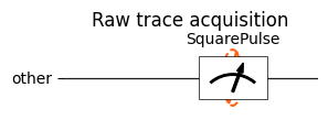
To test the implemented CompilationNode, we first create a raw trace Schedule:

from quantify_scheduler.schedules.trace_schedules import trace_schedule

sched = trace_schedule(
    pulse_amp=0.1,
    pulse_duration=1e-7,
    pulse_delay=0,
    frequency=3e9,
    acquisition_delay=0,
    integration_time=2e-7,
    port="q0:res",
    clock="q0.ro"
)
sched.plot_circuit_diagram()

(<Figure size 1000x100 with 1 Axes>,
 <Axes: title={'center': 'Raw trace acquisition'}>)

Currently, the QuantumDevice is responsible for generating the full CompilationConfig. We therefore create an empty QuantumDevice:

from quantify_scheduler.device_under_test.quantum_device import QuantumDevice

quantum_device = QuantumDevice("quantum_device")

We supply the hardware compilation config input to the QuantumDevice, which will be used to generate the full CompilationConfig:

from quantify_scheduler.backends.mock.mock_rom import hardware_compilation_config as hw_cfg
quantum_device.hardware_config(hw_cfg)

The QuantumDevice can now generate the full CompilationConfig:

from rich import print

print(quantum_device.generate_compilation_config())

SerialCompilationConfig(
    name='QuantumDevice-generated SerialCompilationConfig',
    version='v0.6',
    keep_original_schedule=True,
    backend=<class 'quantify_scheduler.backends.graph_compilation.SerialCompiler'>,
    device_compilation_config=DeviceCompilationConfig(
        clocks={},
        elements={},
        edges={},
        scheduling_strategy=<SchedulingStrategy.ASAP: 'asap'>,
        compilation_passes=[
            SimpleNodeConfig(
                name='circuit_to_device',
                compilation_func=<function compile_circuit_to_device_with_config_validation at 0x7d2537c543a0>
            ),
            SimpleNodeConfig(
                name='set_pulse_and_acquisition_clock',
                compilation_func=<function set_pulse_and_acquisition_clock at 0x7d2537c544c0>
            ),
            SimpleNodeConfig(
                name='process_compensation_pulses',
                compilation_func=<function process_compensation_pulses at 0x7d2537c61670>
            ),
            SimpleNodeConfig(
                name='determine_absolute_timing',
                compilation_func=<function _determine_absolute_timing at 0x7d2537cc4af0>
            ),
            SimpleNodeConfig(
                name='normalize_absolute_timing',
                compilation_func=<function _normalize_absolute_timing at 0x7d2537ccb160>
            )
        ]
    ),
    hardware_compilation_config=MockROMHardwareCompilationConfig(
        config_type=<class 'quantify_scheduler.backends.mock.mock_rom.MockROMHardwareCompilationConfig'>,
        hardware_description={
            'mock_rom': MockROMDescription(instrument_type='Mock readout module', sampling_rate=1500000000.0)
        },
        hardware_options=MockROMHardwareOptions(
            crosstalk=None,
            latency_corrections=None,
            distortion_corrections=None,
            modulation_frequencies={'q0:res-q0.ro': ModulationFrequencies(interm_freq=100000000.0, lo_freq=None)},
            mixer_corrections=None,
            gain={'q0:res-q0.ro': 2.0}
        ),
        connectivity=Connectivity(graph=<quantify_scheduler.structure.types.Graph object at 0x7d2537d145e0>),
        compilation_passes=[
            SimpleNodeConfig(
                name='mock_rom_hardware_compile',
                compilation_func=<function hardware_compile at 0x7d2540222c10>
            )
        ]
    ),
    debug_mode=False
)

We can now compile the Schedule to settings for the mock readout module:

from quantify_scheduler.backends.graph_compilation import SerialCompiler

compiler = SerialCompiler(name="compiler", quantum_device=quantum_device)
compiled_schedule = compiler.compile(schedule=sched)

We can now check that the compiled settings are correct:

print(compiled_schedule.compiled_instructions)

{
    'mock_rom': MockROMSettings(
        waveforms={
            '2504548127482192098_I': NDArray([ 0.1       ,  0.09135455,  0.06691306,  0.0309017 , -0.01045285,
         -0.05      , -0.0809017 , -0.09781476, -0.09781476, -0.0809017 ,
         -0.05      , -0.01045285,  0.0309017 ,  0.06691306,  0.09135455,
          0.1       ,  0.09135455,  0.06691306,  0.0309017 , -0.01045285,
         -0.05      , -0.0809017 , -0.09781476, -0.09781476, -0.0809017 ,
         -0.05      , -0.01045285,  0.0309017 ,  0.06691306,  0.09135455,
          0.1       ,  0.09135455,  0.06691306,  0.0309017 , -0.01045285,
         -0.05      , -0.0809017 , -0.09781476, -0.09781476, -0.0809017 ,
         -0.05      , -0.01045285,  0.0309017 ,  0.06691306,  0.09135455,
          0.1       ,  0.09135455,  0.06691306,  0.0309017 , -0.01045285,
         -0.05      , -0.0809017 , -0.09781476, -0.09781476, -0.0809017 ,
         -0.05      , -0.01045285,  0.0309017 ,  0.06691306,  0.09135455,
          0.1       ,  0.09135455,  0.06691306,  0.0309017 , -0.01045285,
         -0.05      , -0.0809017 , -0.09781476, -0.09781476, -0.0809017 ,
         -0.05      , -0.01045285,  0.0309017 ,  0.06691306,  0.09135455,
          0.1       ,  0.09135455,  0.06691306,  0.0309017 , -0.01045285,
         -0.05      , -0.0809017 , -0.09781476, -0.09781476, -0.0809017 ,
         -0.05      , -0.01045285,  0.0309017 ,  0.06691306,  0.09135455,
          0.1       ,  0.09135455,  0.06691306,  0.0309017 , -0.01045285,
         -0.05      , -0.0809017 , -0.09781476, -0.09781476, -0.0809017 ,
         -0.05      , -0.01045285,  0.0309017 ,  0.06691306,  0.09135455,
          0.1       ,  0.09135455,  0.06691306,  0.0309017 , -0.01045285,
         -0.05      , -0.0809017 , -0.09781476, -0.09781476, -0.0809017 ,
         -0.05      , -0.01045285,  0.0309017 ,  0.06691306,  0.09135455,
          0.1       ,  0.09135455,  0.06691306,  0.0309017 , -0.01045285,
         -0.05      , -0.0809017 , -0.09781476, -0.09781476, -0.0809017 ,
         -0.05      , -0.01045285,  0.0309017 ,  0.06691306,  0.09135455,
          0.1       ,  0.09135455,  0.06691306,  0.0309017 , -0.01045285,
         -0.05      , -0.0809017 , -0.09781476, -0.09781476, -0.0809017 ,
         -0.05      , -0.01045285,  0.0309017 ,  0.06691306,  0.09135455]),
            '2504548127482192098_Q': NDArray([ 0.00000000e+00,  4.06736643e-02,  7.43144825e-02,
          9.51056516e-02,  9.94521895e-02,  8.66025404e-02,
          5.87785252e-02,  2.07911691e-02, -2.07911691e-02,
         -5.87785252e-02, -8.66025404e-02, -9.94521895e-02,
         -9.51056516e-02, -7.43144825e-02, -4.06736643e-02,
         -2.44929360e-17,  4.06736643e-02,  7.43144825e-02,
          9.51056516e-02,  9.94521895e-02,  8.66025404e-02,
          5.87785252e-02,  2.07911691e-02, -2.07911691e-02,
         -5.87785252e-02, -8.66025404e-02, -9.94521895e-02,
         -9.51056516e-02, -7.43144825e-02, -4.06736643e-02,
         -4.89858720e-17,  4.06736643e-02,  7.43144825e-02,
          9.51056516e-02,  9.94521895e-02,  8.66025404e-02,
          5.87785252e-02,  2.07911691e-02, -2.07911691e-02,
         -5.87785252e-02, -8.66025404e-02, -9.94521895e-02,
         -9.51056516e-02, -7.43144825e-02, -4.06736643e-02,
         -4.28750176e-16,  4.06736643e-02,  7.43144825e-02,
          9.51056516e-02,  9.94521895e-02,  8.66025404e-02,
          5.87785252e-02,  2.07911691e-02, -2.07911691e-02,
         -5.87785252e-02, -8.66025404e-02, -9.94521895e-02,
         -9.51056516e-02, -7.43144825e-02, -4.06736643e-02,
         -9.79717439e-17,  4.06736643e-02,  7.43144825e-02,
          9.51056516e-02,  9.94521895e-02,  8.66025404e-02,
          5.87785252e-02,  2.07911691e-02, -2.07911691e-02,
         -5.87785252e-02, -8.66025404e-02, -9.94521895e-02,
         -9.51056516e-02, -7.43144825e-02, -4.06736643e-02,
         -4.77736048e-16,  4.06736643e-02,  7.43144825e-02,
          9.51056516e-02,  9.94521895e-02,  8.66025404e-02,
          5.87785252e-02,  2.07911691e-02, -2.07911691e-02,
         -5.87785252e-02, -8.66025404e-02, -9.94521895e-02,
         -9.51056516e-02, -7.43144825e-02, -4.06736643e-02,
         -8.57500352e-16,  4.06736643e-02,  7.43144825e-02,
          9.51056516e-02,  9.94521895e-02,  8.66025404e-02,
          5.87785252e-02,  2.07911691e-02, -2.07911691e-02,
         -5.87785252e-02, -8.66025404e-02, -9.94521895e-02,
         -9.51056516e-02, -7.43144825e-02, -4.06736643e-02,
         -8.81993288e-16,  4.06736643e-02,  7.43144825e-02,
          9.51056516e-02,  9.94521895e-02,  8.66025404e-02,
          5.87785252e-02,  2.07911691e-02, -2.07911691e-02,
         -5.87785252e-02, -8.66025404e-02, -9.94521895e-02,
         -9.51056516e-02, -7.43144825e-02, -4.06736643e-02,
         -1.95943488e-16,  4.06736643e-02,  7.43144825e-02,
          9.51056516e-02,  9.94521895e-02,  8.66025404e-02,
          5.87785252e-02,  2.07911691e-02, -2.07911691e-02,
         -5.87785252e-02, -8.66025404e-02, -9.94521895e-02,
         -9.51056516e-02, -7.43144825e-02, -4.06736643e-02,
         -9.30979160e-16,  4.06736643e-02,  7.43144825e-02,
          9.51056516e-02,  9.94521895e-02,  8.66025404e-02,
          5.87785252e-02,  2.07911691e-02, -2.07911691e-02,
         -5.87785252e-02, -8.66025404e-02, -9.94521895e-02,
         -9.51056516e-02, -7.43144825e-02, -4.06736643e-02])
        },
        instructions=['TRACE_input0_0'],
        sampling_rate=1500000000.0,
        gain=2.0,
        acq_channels_data={
            0: AcquisitionChannelData(
                acq_index_dim_name='acq_index_0',
                protocol='Trace',
                bin_mode=<BinMode.AVERAGE: 'average'>,
                coords={}
            )
        },
        hardware_acq_mapping_trace={0: 0},
        hardware_acq_mapping_binned={}
    )
}

5. Integration with the ScheduleGettable

The ScheduleGettable integrates the InstrumentCoordinatorComponents with the QuantifyCompiler to provide a straightforward interface for the user to execute a Schedule on the hardware and retrieve the acquired data. The ScheduleGettable takes a QuantumDevice and a Schedule as input and returns the data from the acquisitions in the Schedule.

Note

This is also mainly a validation step. If we did everything correctly, no new development should be needed in this step.

We first instantiate the InstrumentCoordinator, add the InstrumentCoordinatorComponent for the mock readout module, and add a reference to the InstrumentCoordinator to the QuantumDevice:

from quantify_scheduler.instrument_coordinator.instrument_coordinator import InstrumentCoordinator

ic = InstrumentCoordinator("IC")
ic.add_component(rom_icc)
quantum_device.instr_instrument_coordinator(ic.name)

We then create a ScheduleGettable:

from quantify_scheduler.gettables import ScheduleGettable
from quantify_scheduler.schedules.trace_schedules import trace_schedule

schedule_gettable = ScheduleGettable(
    quantum_device=quantum_device,
    schedule_function=trace_schedule,
    schedule_kwargs=dict(
        pulse_amp=0.1,
        pulse_duration=1e-7,
        pulse_delay=0,
        frequency=3e9,
        acquisition_delay=0,
        integration_time=2e-7,
        port="q0:res",
        clock="q0.ro"
    ),
    batched=True
)
I, Q = schedule_gettable.get()

We can now plot the acquired data:

plt.plot(I)
plt.plot(Q)
plt.show()

6. Integration with the MeasurementControl

Note

This is mainly a validation step. If we did everything correctly, no new development should be needed in this step.

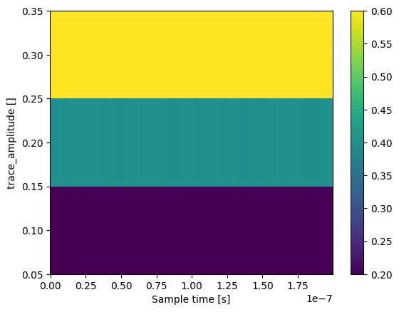
Example of a MeasurementControl that sweeps the pulse amplitude in the trace ScheduleGettable:

from quantify_core.measurement.control import MeasurementControl
from quantify_core.data.handling import set_datadir, to_gridded_dataset

set_datadir()

meas_ctrl = MeasurementControl(name="meas_ctrl")

from qcodes.parameters import ManualParameter

amp_par = ManualParameter(name="trace_amplitude")
amp_par.batched = False
sample_par = ManualParameter("sample", label="Sample time", unit="s")
sample_par.batched = True

amps = [0.1,0.2,0.3]
integration_time = 2e-7
sampling_rate = quantum_device.generate_hardware_compilation_config().hardware_description["mock_rom"].sampling_rate

schedule_gettable = ScheduleGettable(
    quantum_device=quantum_device,
    schedule_function=trace_schedule,
    schedule_kwargs=dict(
        pulse_amp=amp_par,
        pulse_duration=1e-7,
        pulse_delay=0,
        frequency=3e9,
        acquisition_delay=0,
        integration_time=integration_time,
        port="q0:res",
        clock="q0.ro"
    ),
    batched=True
)
meas_ctrl.settables([amp_par, sample_par])
# problem: we don't necessarily know the size of the returned traces (solved by using xarray?)
# workaround: use sample_par ManualParameter that predicts this using the sampling rate
meas_ctrl.setpoints_grid([np.array(amps), np.arange(0, integration_time, 1 / sampling_rate)])
meas_ctrl.gettables(schedule_gettable)

data = meas_ctrl.run()
gridded_data = to_gridded_dataset(data)

Data will be saved in:
/root/quantify-data
Starting batched measurement...
Iterative settable(s) [outer loop(s)]:
	 trace_amplitude 
Batched settable(s):
	 sample 
Batch size limit: 900

Data processing and plotting:

import xarray as xr

magnitude_data = abs(gridded_data.y0 + 1j * gridded_data.y1)
phase_data = xr.DataArray(np.angle(gridded_data.y0 + 1j * gridded_data.y1))

magnitude_data.plot()

<matplotlib.collections.QuadMesh at 0x7d25366a7b20>

phase_data.plot()

<matplotlib.collections.QuadMesh at 0x7d25365de9d0>

7. Binned acquisition

Above, we implemented the trace acquisition protocol in our mock backend. In this section we implement a binned acquisition. Binned acquisitions are more complicated, because

1. multiple operations can use the same acquisition channel, for example

schedule = Schedule("example")
schedule.add(SSBIntegrationComplex(acq_channel="ch_0", coords={"freq": 100}))
schedule.add(SSBIntegrationComplex(acq_channel="ch_0", coords={"freq": 200}))

2. the same operation can be used for multiple acquisitions, for example when the exact same operation is added to the schedule as different schedulables,

schedule = Schedule("example")

acquisition = SSBIntegrationComplex(acq_channel="ch_0")

schedule.add(acquisition)
schedule.add(acquisition)

The data the user receives is a 1 dimensional xarray.DataArray for each acquisition channel (assuming no append mode repetitions), indexed by acquisition index. If unspecified by the user, the acquisition index is autogenerated by generate_acq_channels_data(). The ultimate goal of the backend is to map each acquisition index to an acquired data from the hardware.

First let’s understand what generate_acq_channels_data() returns.

from quantify_scheduler.schedules.schedule import Schedule
from quantify_scheduler.operations.acquisition_library import SSBIntegrationComplex
from quantify_scheduler.helpers.generate_acq_channels_data import generate_acq_channels_data
from quantify_scheduler.compilation import _determine_absolute_timing

schedule = Schedule("example")

subschedule = Schedule("subschedule")
subschedule.add(
    SSBIntegrationComplex(
        acq_channel="ch_0",
        coords={"amp": 0.1},
        acq_index=None,
        bin_mode=BinMode.AVERAGE,
        port="q0:res",
        clock="q0.01",
        duration=100e-9
    )
)

schedule.add(subschedule)
schedule.add(subschedule)

schedule = _determine_absolute_timing(schedule)

acq_channels_data, schedulable_to_acq_index = generate_acq_channels_data(schedule)
acq_channels_data, schedulable_to_acq_index

({'ch_0': AcquisitionChannelData(acq_index_dim_name='acq_index_ch_0', protocol='SSBIntegrationComplex', bin_mode=<BinMode.AVERAGE: 'average'>, coords=[{'amp': 0.1}, {'amp': 0.1}])},
 {(('ac419bb2-2f3d-4dd7-af7d-723032d5882e',
    'a98cdd98-3dff-4144-b9ea-cf75db5407c9'),
   0): 0,
  (('8c1fa6a8-a459-40eb-b346-7a1a8427f918',
    'a98cdd98-3dff-4144-b9ea-cf75db5407c9'),
   0): 1})

In the example schedule, there are two acquisitions, so for acquisition channel "ch_0" two acquisition indices are generated: the coords has 2 elements. The generated acquisition indices are not explicitly written out in acq_channels_data, they’re just the indices of the coords.

The backends job is to map each acquisition to a hardware acquisition data, but unfortunately, if the compiler added the acquisition index to the operation, that would be incorrect, because there is only one operation, but two acquisition indices. Therefore, generate_acq_channels_data() maps each schedulable label to an acquisition index. To be more precise, it maps the tuple of the schedulable of the subschedule and schedulable of the acquisition operation to the acquisition index. (Also, there’s an acquisition info at the end (0), because multiple acquisition info might be present, with possibly different acquisition indices.) Note: using schedulables instead of operations to reference acquisitions can also be important for loops, and other control flow structures.

Our mock hardware does binned acquisition with the "ACQ_input0_0" instruction where input0 is the hardware port and the 0 at the end is the “bin” for that acquisition. The backend compiler maps each schedulable to a bin. hardware_compile() generates this mapping, using SchedulableLabelToAcquisitionIndex.

from quantify_scheduler.schedules.schedule import Schedule
from quantify_scheduler.operations.acquisition_library import SSBIntegrationComplex, Trace
from quantify_scheduler.compilation import _determine_absolute_timing
from quantify_scheduler.backends.mock.mock_rom import hardware_compile
from quantify_scheduler.resources import ClockResource
from quantify_scheduler.operations.pulse_library import SquarePulse

schedule = Schedule("example")

schedule.add_resource(ClockResource("q0.ro", 3e9))

schedule.add(SquarePulse(duration=100e-9, amp=0.1, port="q0:res", clock="q0.ro"))
schedule.add(Trace(acq_channel="ch_trace", duration=100e-9, port="q0:res", clock="q0.ro"))

schedule.add(
    SSBIntegrationComplex(
        acq_channel="ch_0",
        coords={"freq": 100},
        acq_index=None,
        bin_mode=BinMode.AVERAGE,
        port="q0:res",
        clock="q0.01",
        duration=100e-9
    )
)
schedule.add(
    SSBIntegrationComplex(
        acq_channel="ch_0",
        coords={"freq": 200},
        acq_index=None,
        bin_mode=BinMode.AVERAGE,
        port="q0:res",
        clock="q0.01",
        duration=100e-9
    )
)

Show code cell output

Hide code cell output

{'name': '7910f1e7-1325-4e1a-8f70-841e6310c573', 'operation_id': '2487560947645639081', 'timing_constraints': [TimingConstraint(ref_schedulable=None, ref_pt=None, ref_pt_new=None, rel_time=0)], 'label': '7910f1e7-1325-4e1a-8f70-841e6310c573'}

This example schedule has two binned acquisitions, both on the same acquisition channel, so we expect that the generate_acq_channels_data() function generates two acquisition index and related coordinates.

schedule = _determine_absolute_timing(schedule)

acq_channels_data, schedulable_to_acq_index = generate_acq_channels_data(schedule)
acq_channels_data, schedulable_to_acq_index

({'ch_trace': AcquisitionChannelData(acq_index_dim_name='acq_index_ch_trace', protocol='Trace', bin_mode=<BinMode.AVERAGE: 'average'>, coords={}),
  'ch_0': AcquisitionChannelData(acq_index_dim_name='acq_index_ch_0', protocol='SSBIntegrationComplex', bin_mode=<BinMode.AVERAGE: 'average'>, coords=[{'freq': 100}, {'freq': 200}])},
 {(('7daab169-ba51-410c-8e39-dc28ef8795b6',), 0): 0,
  (('7910f1e7-1325-4e1a-8f70-841e6310c573',), 0): 1})

Based on this, the hardware backend creates a hardware acquisition mapping.

schedule = _determine_absolute_timing(schedule)

compiled_schedule = hardware_compile(schedule, quantum_device.generate_compilation_config())

compiled_schedule["compiled_instructions"]["mock_rom"].hardware_acq_mapping_binned

{('ch_0', 0): 1, ('ch_0', 1): 2}

This hardware mapping is in the compiled schedule, and later is used to map the hardware data to the xarray.Dataset. In practice, each acquisition channel and acquisition index is mapped to a hardware bin.

There are a set of utility functions that help backend developers to format the retrieved data: add_acquisition_coords_binned() and add_acquisition_coords_nonbinned(). The mock backend calls these functions to add the “coords” to the retrieved data before returning it to users.

The retrieved data includes both acquisition indices and coords on the relevant acquisition channel, and does not contain the hardware bins.

settings = compiled_schedule["compiled_instructions"]["mock_rom"]
rom_icc.prepare(settings)
rom_icc.start()
rom_icc.retrieve_acquisition()

<xarray.Dataset> Size: 4kB
Dimensions:             (acq_index_ch_trace: 1, time_ch_trace: 150,
                         acq_index_ch_0: 2)
Coordinates:
  * acq_index_ch_trace  (acq_index_ch_trace) int64 8B 0
  * time_ch_trace       (time_ch_trace) float64 1kB 0.0 1e-09 ... 1.49e-07
  * acq_index_ch_0      (acq_index_ch_0) int64 16B 0 1
    freq                (acq_index_ch_0) float64 16B 100.0 200.0
Data variables:
    ch_trace            (acq_index_ch_trace, time_ch_trace) complex128 2kB (0...
    ch_0                (acq_index_ch_0) float64 16B 0.04007 0.3334

xarray.Dataset

• Dimensions:
  • acq_index_ch_trace: 1
  • time_ch_trace: 150
  • acq_index_ch_0: 2
• Coordinates: (4)
  • acq_index_ch_trace
    (acq_index_ch_trace)
    int64
    0

    array([0])

  • time_ch_trace
    (time_ch_trace)
    float64
    0.0 1e-09 ... 1.48e-07 1.49e-07

    array([0.00e+00, 1.00e-09, 2.00e-09, 3.00e-09, 4.00e-09, 5.00e-09, 6.00e-09,
           7.00e-09, 8.00e-09, 9.00e-09, 1.00e-08, 1.10e-08, 1.20e-08, 1.30e-08,
           1.40e-08, 1.50e-08, 1.60e-08, 1.70e-08, 1.80e-08, 1.90e-08, 2.00e-08,
           2.10e-08, 2.20e-08, 2.30e-08, 2.40e-08, 2.50e-08, 2.60e-08, 2.70e-08,
           2.80e-08, 2.90e-08, 3.00e-08, 3.10e-08, 3.20e-08, 3.30e-08, 3.40e-08,
           3.50e-08, 3.60e-08, 3.70e-08, 3.80e-08, 3.90e-08, 4.00e-08, 4.10e-08,
           4.20e-08, 4.30e-08, 4.40e-08, 4.50e-08, 4.60e-08, 4.70e-08, 4.80e-08,
           4.90e-08, 5.00e-08, 5.10e-08, 5.20e-08, 5.30e-08, 5.40e-08, 5.50e-08,
           5.60e-08, 5.70e-08, 5.80e-08, 5.90e-08, 6.00e-08, 6.10e-08, 6.20e-08,
           6.30e-08, 6.40e-08, 6.50e-08, 6.60e-08, 6.70e-08, 6.80e-08, 6.90e-08,
           7.00e-08, 7.10e-08, 7.20e-08, 7.30e-08, 7.40e-08, 7.50e-08, 7.60e-08,
           7.70e-08, 7.80e-08, 7.90e-08, 8.00e-08, 8.10e-08, 8.20e-08, 8.30e-08,
           8.40e-08, 8.50e-08, 8.60e-08, 8.70e-08, 8.80e-08, 8.90e-08, 9.00e-08,
           9.10e-08, 9.20e-08, 9.30e-08, 9.40e-08, 9.50e-08, 9.60e-08, 9.70e-08,
           9.80e-08, 9.90e-08, 1.00e-07, 1.01e-07, 1.02e-07, 1.03e-07, 1.04e-07,
           1.05e-07, 1.06e-07, 1.07e-07, 1.08e-07, 1.09e-07, 1.10e-07, 1.11e-07,
           1.12e-07, 1.13e-07, 1.14e-07, 1.15e-07, 1.16e-07, 1.17e-07, 1.18e-07,
           1.19e-07, 1.20e-07, 1.21e-07, 1.22e-07, 1.23e-07, 1.24e-07, 1.25e-07,
           1.26e-07, 1.27e-07, 1.28e-07, 1.29e-07, 1.30e-07, 1.31e-07, 1.32e-07,
           1.33e-07, 1.34e-07, 1.35e-07, 1.36e-07, 1.37e-07, 1.38e-07, 1.39e-07,
           1.40e-07, 1.41e-07, 1.42e-07, 1.43e-07, 1.44e-07, 1.45e-07, 1.46e-07,
           1.47e-07, 1.48e-07, 1.49e-07])

  • acq_index_ch_0
    (acq_index_ch_0)
    int64
    0 1

    array([0, 1])

  • freq
    (acq_index_ch_0)
    float64
    100.0 200.0

    array([100., 200.])

• Data variables: (2)
  • ch_trace
    (acq_index_ch_trace, time_ch_trace)
    complex128
    (0.2+0j) ... (0.1827090915285192...

    acq_protocol :

    Trace

    array([[ 0.2       +0.00000000e+00j,  0.18270909+8.13473286e-02j,
             0.13382612+1.48628965e-01j,  0.0618034 +1.90211303e-01j,
            -0.02090569+1.98904379e-01j, -0.1       +1.73205081e-01j,
            -0.1618034 +1.17557050e-01j, -0.19562952+4.15823382e-02j,
            -0.19562952-4.15823382e-02j, -0.1618034 -1.17557050e-01j,
            -0.1       -1.73205081e-01j, -0.02090569-1.98904379e-01j,
             0.0618034 -1.90211303e-01j,  0.13382612-1.48628965e-01j,
             0.18270909-8.13473286e-02j,  0.2       -4.89858720e-17j,
             0.18270909+8.13473286e-02j,  0.13382612+1.48628965e-01j,
             0.0618034 +1.90211303e-01j, -0.02090569+1.98904379e-01j,
            -0.1       +1.73205081e-01j, -0.1618034 +1.17557050e-01j,
            -0.19562952+4.15823382e-02j, -0.19562952-4.15823382e-02j,
            -0.1618034 -1.17557050e-01j, -0.1       -1.73205081e-01j,
            -0.02090569-1.98904379e-01j,  0.0618034 -1.90211303e-01j,
             0.13382612-1.48628965e-01j,  0.18270909-8.13473286e-02j,
             0.2       -9.79717439e-17j,  0.18270909+8.13473286e-02j,
             0.13382612+1.48628965e-01j,  0.0618034 +1.90211303e-01j,
            -0.02090569+1.98904379e-01j, -0.1       +1.73205081e-01j,
            -0.1618034 +1.17557050e-01j, -0.19562952+4.15823382e-02j,
            -0.19562952-4.15823382e-02j, -0.1618034 -1.17557050e-01j,
    ...
            -0.1       +1.73205081e-01j, -0.1618034 +1.17557050e-01j,
            -0.19562952+4.15823382e-02j, -0.19562952-4.15823382e-02j,
            -0.1618034 -1.17557050e-01j, -0.1       -1.73205081e-01j,
            -0.02090569-1.98904379e-01j,  0.0618034 -1.90211303e-01j,
             0.13382612-1.48628965e-01j,  0.18270909-8.13473286e-02j,
             0.2       -3.91886976e-16j,  0.18270909+8.13473286e-02j,
             0.13382612+1.48628965e-01j,  0.0618034 +1.90211303e-01j,
            -0.02090569+1.98904379e-01j, -0.1       +1.73205081e-01j,
            -0.1618034 +1.17557050e-01j, -0.19562952+4.15823382e-02j,
            -0.19562952-4.15823382e-02j, -0.1618034 -1.17557050e-01j,
            -0.1       -1.73205081e-01j, -0.02090569-1.98904379e-01j,
             0.0618034 -1.90211303e-01j,  0.13382612-1.48628965e-01j,
             0.18270909-8.13473286e-02j,  0.2       -1.86195832e-15j,
             0.18270909+8.13473286e-02j,  0.13382612+1.48628965e-01j,
             0.0618034 +1.90211303e-01j, -0.02090569+1.98904379e-01j,
            -0.1       +1.73205081e-01j, -0.1618034 +1.17557050e-01j,
            -0.19562952+4.15823382e-02j, -0.19562952-4.15823382e-02j,
            -0.1618034 -1.17557050e-01j, -0.1       -1.73205081e-01j,
            -0.02090569-1.98904379e-01j,  0.0618034 -1.90211303e-01j,
             0.13382612-1.48628965e-01j,  0.18270909-8.13473286e-02j]])

  • ch_0
    (acq_index_ch_0)
    float64
    0.04007 0.3334

    acq_protocol :

    SSBIntegrationComplex

    array([0.04007487, 0.33340943])

• Indexes: (3)
  • acq_index_ch_trace
    PandasIndex

    PandasIndex(Index([0], dtype='int64', name='acq_index_ch_trace'))

  • time_ch_trace
    PandasIndex

    PandasIndex(Index([                   0.0,                  1e-09,                  2e-09,
           3.0000000000000004e-09,                  4e-09,                  5e-09,
            6.000000000000001e-09,  7.000000000000001e-09,                  8e-09,
            9.000000000000001e-09,
           ...
                          1.4e-07,               1.41e-07,               1.42e-07,
                         1.43e-07, 1.4400000000000002e-07, 1.4500000000000001e-07,
                         1.46e-07,               1.47e-07,               1.48e-07,
                         1.49e-07],
          dtype='float64', name='time_ch_trace', length=150))

  • acq_index_ch_0
    PandasIndex

    PandasIndex(Index([0, 1], dtype='int64', name='acq_index_ch_0'))

• Attributes: (0)