schedule#

Module containing the core concepts of the scheduler.

Module Contents#

Classes#

`ScheduleBase`	Interface to be used for `Schedule`.
`Schedule`	A modifiable schedule.
`Schedulable`	A representation of an element on a schedule.
`AcquisitionChannelData`	Datastructure to store metadata for the given acquisition channel.
`CompiledSchedule`	A schedule that contains compiled instructions ready for execution using the `InstrumentCoordinator`.
`AcquisitionChannelMetadata`	A description of the acquisition channel and it's indices.
`AcquisitionMetadata`	A description of the shape and type of data that a schedule will return when executed.

Attributes#

`DictOrdered`	An ordered dictionary type hint,
`AcquisitionChannelsData`	Dictionary mapping each acq_channel to their corresponding

DictOrdered[source]#: An ordered dictionary type hint, which makes it clear and obvious that order is significant and used by the logic. Note: dict is ordered from Python version 3.7. Note: collections.OrderedDict can be slow in some cases.

class ScheduleBase(dict=None, /, **kwargs)[source]#

Bases: quantify_scheduler.json_utils.JSONSchemaValMixin, quantify_scheduler.json_utils.JSONSerializableMixin, collections.UserDict, abc.ABC

Interface to be used for Schedule.

The ScheduleBase is a data structure that is at the core of the Quantify-scheduler and describes when what operations are applied where.

The ScheduleBase is a collection of quantify_scheduler.operations.operation.Operation objects and timing constraints that define relations between the operations.

The schedule data structure is based on a dictionary. This dictionary contains:

operation_dict - a hash table containing the unique
quantify_scheduler.operations.operation.Operation s added to the schedule.
schedulables - an ordered dictionary of all timing constraints added
between operations; when multiple schedulables have the same absolute time, the order defined in the dictionary decides precedence.

The Schedule provides an API to create schedules. The CompiledSchedule represents a schedule after it has been compiled for execution on a backend.

The Schedule contains information on the operations and schedulables. The operations is a dictionary of all unique operations used in the schedule and contain the information on what operation to apply where. The schedulables is a dictionary of Schedulables describing timing constraints between operations, i.e. when to apply an operation.

JSON schema of a valid Schedule

JSON schema for a quantify schedule.
type	object
properties
name	Name of the schedule.
	type	string
repetitions	The amount of times the schedule will be repeated.
	type	integer
	default	1
schedulables	An ordered dictionary containing schedulables.
	type	object
operation_dict	A dictionary of operations. Keys correspond to the hash attribute of operations.
	type	object
resource_dict	A dictionary of resources.
	type	object
compiled_instructions	A MutableMapping object containing compiled instructions.
duration	Duration of the schedule.
	type	number
acq_channels_data	A dictionary containing data for every acquisition channel.
	type	object
additionalProperties	False

property name: str[source]#: Returns the name of the schedule.

property repetitions: int[source]#

Returns the amount of times this Schedule will be repeated.

Returns:

: The repetitions count.

property operations: dict[str, quantify_scheduler.operations.operation.Operation | Schedule][source]#

A dictionary of all unique operations used in the schedule.

This specifies information on what operation to apply where.

The keys correspond to the hash and values are instances of quantify_scheduler.operations.operation.Operation.

property schedulables: DictOrdered[str, Schedulable][source]#

Ordered dictionary of schedulables describing timing and order of operations.

A schedulable uses timing constraints to constrain the operation in time by specifying the time ("rel_time") between a reference operation and the added operation. The time can be specified with respect to a reference point ("ref_pt"') on the reference operation (:code:”ref_op”) and a reference point on the next added operation (:code:”ref_pt_new”’). A reference point can be either the “start”, “center”, or “end” of an operation. The reference operation ("ref_op") is specified using its label property.

Each item in the list represents a timing constraint and is a dictionary with the following keys:

['label', 'rel_time', 'ref_op', 'ref_pt_new', 'ref_pt', 'operation_id']

The label is used as a unique identifier that can be used as a reference for other operations, the operation_id refers to the hash of an operation in operations.

Note

timing constraints are not intended to be modified directly. Instead use the add()

property resources: dict[str, quantify_scheduler.resources.Resource][source]#

A dictionary containing resources.

Keys are names (str), values are instances of Resource.

property hash: str[source]#: A hash based on the contents of the Schedule.

get_used_port_clocks() → set[tuple[str, str]][source]#

Extracts which port-clock combinations are used in this schedule.

Returns:

: All (port, clock) combinations that operations in this schedule uses

plot_circuit_diagram(figsize: tuple[int, int] | None = None, ax: matplotlib.axes.Axes | None = None, plot_backend: Literal['mpl'] = 'mpl') → tuple[matplotlib.figure.Figure, matplotlib.axes.Axes | list[matplotlib.axes.Axes]][source]#

Create a circuit diagram visualization of the schedule using the specified plotting backend.

The circuit diagram visualization depicts the schedule at the quantum circuit layer. Because quantify-scheduler uses a hybrid gate-pulse paradigm, operations for which no information is specified at the gate level are visualized using an icon (e.g., a stylized wavy pulse) depending on the information specified at the quantum device layer.

Alias of quantify_scheduler.schedules._visualization.circuit_diagram.circuit_diagram_matplotlib().

Parameters:

schedule – the schedule to render.
figsize – matplotlib figsize.
ax – Axis handle to use for plotting.
plot_backend – Plotting backend to use, currently only ‘mpl’ is supported

Returns:

fig: matplotlib figure object.
ax: matplotlib axis object.

Each gate, pulse, measurement, and any other operation are plotted in the order of execution, but no timing information is provided.

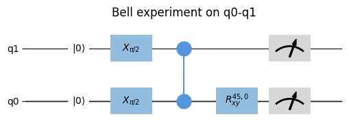
Example

from quantify_scheduler import Schedule
from quantify_scheduler.operations.gate_library import Reset, X90, CZ, Rxy, Measure

sched = Schedule(f"Bell experiment on q0-q1")

sched.add(Reset("q0", "q1"))
sched.add(X90("q0"))
sched.add(X90("q1"), ref_pt="start", rel_time=0)
sched.add(CZ(qC="q0", qT="q1"))
sched.add(Rxy(theta=45, phi=0, qubit="q0") )
sched.add(Measure("q0", acq_index=0))
sched.add(Measure("q1", acq_index=0), ref_pt="start")

sched.plot_circuit_diagram();

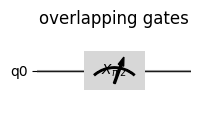
Note

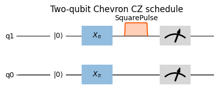
Gates that are started simultaneously on the same qubit will overlap.

from quantify_scheduler import Schedule
from quantify_scheduler.operations.gate_library import X90, Measure

sched = Schedule(f"overlapping gates")

sched.add(X90("q0"))
sched.add(Measure("q0"), ref_pt="start", rel_time=0)
sched.plot_circuit_diagram();

Note

If the pulse’s port address was not found then the pulse will be plotted on the ‘other’ timeline.

plot_pulse_diagram(port_list: list[str] | None = None, sampling_rate: float = 1000000000.0, modulation: Literal['off', 'if', 'clock'] = 'off', modulation_if: float = 0.0, plot_backend: Literal['mpl', 'plotly'] = 'mpl', x_range: tuple[float, float] = (-np.inf, np.inf), combine_waveforms_on_same_port: bool = False, **backend_kwargs) → tuple[matplotlib.figure.Figure, matplotlib.axes.Axes] | plotly.graph_objects.Figure[source]#

Create a visualization of all the pulses in a schedule using the specified plotting backend.

The pulse diagram visualizes the schedule at the quantum device layer. For this visualization to work, all operations need to have the information present (e.g., pulse info) to represent these on the quantum-circuit level and requires the absolute timing to have been determined. This information is typically added when the quantum-device level compilation is performed.

Alias of quantify_scheduler.schedules._visualization.pulse_diagram.pulse_diagram_matplotlib() and quantify_scheduler.schedules._visualization.pulse_diagram.pulse_diagram_plotly().

Parameters:

port_list – A list of ports to show. If None (default) the first 8 ports encountered in the sequence are used.
modulation – Determines if modulation is included in the visualization.
modulation_if – Modulation frequency used when modulation is set to “if”.
sampling_rate – The time resolution used to sample the schedule in Hz.
plot_backend – Plotting library to use, can either be ‘mpl’ or ‘plotly’.
x_range – The range of the x-axis that is plotted, given as a tuple (left limit, right limit). This can be used to reduce memory usage when plotting a small section of a long pulse sequence. By default (-np.inf, np.inf).
combine_waveforms_on_same_port – By default False. If True, combines all waveforms on the same port into one single waveform. The resulting waveform is the sum of all waveforms on that port (small inaccuracies may occur due to floating point approximation). If False, the waveforms are shown individually.
backend_kwargs – Keyword arguments to be passed on to the plotting backend. The arguments that can be used for either backend can be found in the documentation of quantify_scheduler.schedules._visualization.pulse_diagram.pulse_diagram_matplotlib() and quantify_scheduler.schedules._visualization.pulse_diagram.pulse_diagram_plotly().

Returns:

Union[tuple[Figure, Axes], plotly.graph_objects.Figure] the plot

Example

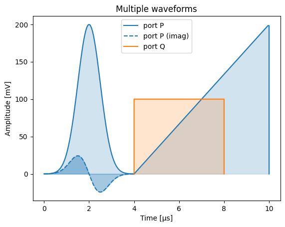
A simple plot with matplotlib can be created as follows:

from quantify_scheduler.backends.graph_compilation import SerialCompiler
from quantify_scheduler.device_under_test.quantum_device import QuantumDevice
from quantify_scheduler.operations.pulse_library import (
    DRAGPulse, SquarePulse, RampPulse, VoltageOffset,
)
from quantify_scheduler.resources import ClockResource

schedule = Schedule("Multiple waveforms")
schedule.add(DRAGPulse(G_amp=0.2, D_amp=0.2, phase=0, duration=4e-6, port="P", clock="C"))
schedule.add(RampPulse(amp=0.2, offset=0.0, duration=6e-6, port="P"))
schedule.add(SquarePulse(amp=0.1, duration=4e-6, port="Q"), ref_pt='start')
schedule.add_resource(ClockResource(name="C", freq=4e9))

quantum_device = QuantumDevice("quantum_device")
device_compiler = SerialCompiler("Device compiler", quantum_device)
compiled_schedule = device_compiler.compile(schedule)

_ = compiled_schedule.plot_pulse_diagram(sampling_rate=20e6)

The backend can be changed to the plotly backend by specifying the plot_backend=plotly argument. With the plotly backend, pulse diagrams include a separate plot for each port/clock combination:

_ = compiled_schedule.plot_pulse_diagram(sampling_rate=20e6, plot_backend='plotly')

The same can be achieved in the default plot_backend (matplotlib) by passing the keyword argument multiple_subplots=True:

_ = compiled_schedule.plot_pulse_diagram(sampling_rate=20e6, multiple_subplots=True)

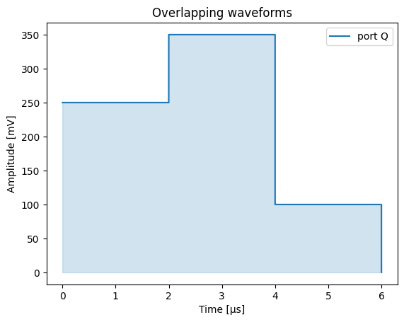
By default, waveforms overlapping in time on the same port are shown separately:

schedule = Schedule("Overlapping waveforms")
schedule.add(VoltageOffset(offset_path_I=0.25, offset_path_Q=0.0, port="Q"))
schedule.add(SquarePulse(amp=0.1, duration=4e-6, port="Q"), rel_time=2e-6)
schedule.add(VoltageOffset(offset_path_I=0.0, offset_path_Q=0.0, port="Q"), ref_pt="start", rel_time=2e-6)

compiled_schedule = device_compiler.compile(schedule)

_ = compiled_schedule.plot_pulse_diagram(sampling_rate=20e6)

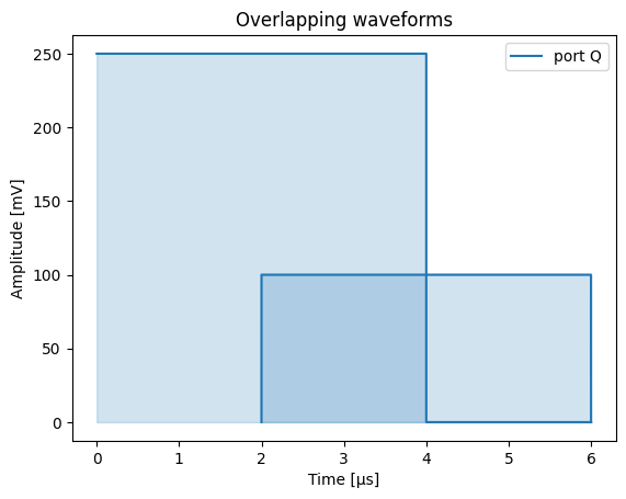
This behaviour can be changed with the parameter combine_waveforms_on_same_port:

_ = compiled_schedule.plot_pulse_diagram(sampling_rate=20e6, combine_waveforms_on_same_port=True)

classmethod _generate_timing_table_list(operation: quantify_scheduler.operations.operation.Operation | ScheduleBase, time_offset: float, timing_table_list: list, operation_id: str | None) → None[source]#

property timing_table: pandas.io.formats.style.Styler[source]#

A styled pandas dataframe containing the absolute timing of pulses and acquisitions in a schedule.

This table is constructed based on the abs_time key in the schedulables. This requires the timing to have been determined.

The table consists of the following columns:

operation: a repr of Operation corresponding to the pulse/acquisition.
waveform_op_id: an id corresponding to each pulse/acquisition inside an Operation.
port: the port the pulse/acquisition is to be played/acquired on.
clock: the clock used to (de)modulate the pulse/acquisition.
abs_time: the absolute time the pulse/acquisition is scheduled to start.
duration: the duration of the pulse/acquisition that is scheduled.
is_acquisition: whether the pulse/acquisition is an acquisition or not (type numpy.bool_).
wf_idx: the waveform index of the pulse/acquisition belonging to the Operation.
operation_hash: the unique hash corresponding to the Schedulable that the pulse/acquisition belongs to.

Example

schedule = Schedule("demo timing table")
schedule.add(Reset("q0", "q4"))
schedule.add(X("q0"))
schedule.add(Y("q4"))
schedule.add(Measure("q0", acq_channel=0, acq_index=0))
schedule.add(Measure("q4", acq_channel=1, acq_index=0))

compiled_schedule = compiler.compile(schedule)
compiled_schedule.timing_table

	waveform_op_id	port	clock	abs_time	duration	is_acquisition	operation	wf_idx	operation_hash
0	Reset('q0','q4')_acq_0	None	cl0.baseband	0.0 ns	200,000.0 ns	False	Reset('q0','q4')	0	666193835919312154
1	Reset('q0','q4')_acq_1	None	cl0.baseband	0.0 ns	200,000.0 ns	False	Reset('q0','q4')	1	666193835919312154
2	X(qubit='q0')_acq_0	q0:mw	q0.01	200,000.0 ns	20.0 ns	False	X(qubit='q0')	0	2516902419063614450
3	Y(qubit='q4')_acq_0	q4:mw	q4.01	200,020.0 ns	20.0 ns	False	Y(qubit='q4')	0	7015308899281260210
4	ResetClockPhase(clock='q0.ro',t0=0)_acq_0	None	q0.ro	200,040.0 ns	0.0 ns	False	ResetClockPhase(clock='q0.ro',t0=0)	0	7665873204631581662
5	SquarePulse(amp=0.25,duration=3e-07,port='q0:res',clock='q0.ro',reference_magnitude=None,t0=0)_acq_0	q0:res	q0.ro	200,040.0 ns	300.0 ns	False	SquarePulse(amp=0.25,duration=3e-07,port='q0:res',clock='q0.ro',reference_magnitude=None,t0=0)	0	6576823774144665149
6	SSBIntegrationComplex(port='q0:res',clock='q0.ro',duration=1e-06,acq_channel=0,acq_index=0,bin_mode='average',phase=0,t0=1e-07)_acq_0	q0:res	q0.ro	200,140.0 ns	1,000.0 ns	True	SSBIntegrationComplex(port='q0:res',clock='q0.ro',duration=1e-06,acq_channel=0,acq_index=0,bin_mode='average',phase=0,t0=1e-07)	0	-8891961521330429897
7	ResetClockPhase(clock='q4.ro',t0=0)_acq_0	None	q4.ro	201,140.0 ns	0.0 ns	False	ResetClockPhase(clock='q4.ro',t0=0)	0	-697958337179229464
8	SquarePulse(amp=0.25,duration=3e-07,port='q4:res',clock='q4.ro',reference_magnitude=None,t0=0)_acq_0	q4:res	q4.ro	201,140.0 ns	300.0 ns	False	SquarePulse(amp=0.25,duration=3e-07,port='q4:res',clock='q4.ro',reference_magnitude=None,t0=0)	0	-9201366481840107066
9	SSBIntegrationComplex(port='q4:res',clock='q4.ro',duration=1e-06,acq_channel=1,acq_index=0,bin_mode='average',phase=0,t0=1e-07)_acq_0	q4:res	q4.ro	201,240.0 ns	1,000.0 ns	True	SSBIntegrationComplex(port='q4:res',clock='q4.ro',duration=1e-06,acq_channel=1,acq_index=0,bin_mode='average',phase=0,t0=1e-07)	0	5878427065319358727

Parameters:

schedule – a schedule for which the absolute timing has been determined.

Returns:

: styled_timing_table, a pandas Styler containing a dataframe with an overview of the timing of the pulses and acquisitions present in the schedule. The dataframe can be accessed through the .data attribute of the Styler.

Raises:

ValueError – When the absolute timing has not been determined during compilation.

get_schedule_duration() → float[source]#

Return the duration of the schedule.

Returns:: schedule_duration : float Duration of current schedule

property duration: float | None[source]#

Determine the cached duration of the schedule.

Will return None if get_schedule_duration() has not been called before.

class Schedule(name: str = 'schedule', repetitions: int = 1, data: dict | None = None)[source]#

Bases: ScheduleBase

A modifiable schedule.

Operations quantify_scheduler.operations.operation.Operation can be added using the add() method, allowing precise specification when to perform an operation using timing constraints.

When adding an operation, it is not required to specify how to represent this quantify_scheduler.operations.operation.Operation on all layers. Instead, this information can be added later during compilation. This allows the user to effortlessly mix the gate- and pulse-level descriptions as required for many (calibration) experiments.

Parameters:

name – The name of the schedule, by default “schedule”
repetitions – The amount of times the schedule will be repeated, by default 1
data – A dictionary containing a pre-existing schedule, by default None

schema_filename = 'schedule.json'[source]#

add_resources(resources_list: list) → None[source]#: Add wrapper for adding multiple resources.

add_resource(resource: quantify_scheduler.resources.Resource) → None[source]#: Add a resource such as a channel or device element to the schedule.

add(operation: quantify_scheduler.operations.operation.Operation | Schedule, rel_time: float = 0, ref_op: Schedulable | str | None = None, ref_pt: Literal['start', 'center', 'end'] | None = None, ref_pt_new: Literal['start', 'center', 'end'] | None = None, label: str | None = None, control_flow: quantify_scheduler.operations.control_flow_library.ControlFlowSpec | None = None) → Schedulable[source]#

Add an operation or a subschedule to the schedule.

Parameters:

operation – The operation to add to the schedule, or another schedule to add as a subschedule.
rel_time – relative time between the reference operation and the added operation. the time is the time between the “ref_pt” in the reference operation and “ref_pt_new” of the operation that is added.
ref_op – reference schedulable. If set to None, will default to the last added operation.
ref_pt – reference point in reference operation must be one of "start", "center", "end", or None; in case of None, _determine_absolute_timing() assumes "end".
ref_pt_new – reference point in added operation must be one of "start", "center", "end", or None; in case of None, _determine_absolute_timing() assumes "start".
label – a unique string that can be used as an identifier when adding operations. if set to None, a random hash will be generated instead.
control_flow – Virtual operation describing if the operation should be subject to control flow (loop, conditional, …). See control flow reference documentation for a detailed explanation.

Returns:

: Returns the schedulable created in the schedule.

_add(operation: quantify_scheduler.operations.operation.Operation | Schedule, rel_time: float = 0, ref_op: Schedulable | str | None = None, ref_pt: Literal['start', 'center', 'end'] | None = None, ref_pt_new: Literal['start', 'center', 'end'] | None = None, label: str | None = None) → Schedulable[source]#

_validate_add_arguments(operation: quantify_scheduler.operations.operation.Operation | Schedule, label: str, control_flow: quantify_scheduler.operations.operation.Operation | None) → None[source]#

class Schedulable(name: str, operation_id: str, control_flow: quantify_scheduler.operations.operation.Operation | None = None)[source]#

Bases: quantify_scheduler.json_utils.JSONSchemaValMixin, collections.UserDict

A representation of an element on a schedule.

All elements on a schedule are schedulables. A schedulable contains all information regarding the timing of this element as well as the operation being executed by this element. This operation is currently represented by an operation ID.

Schedulables can contain an arbitrary number of timing constraints to determine the timing. Multiple different constraints are currently resolved by delaying the element until after all timing constraints have been met, to aid compatibility. To specify an exact timing between two schedulables, please ensure to only specify exactly one timing constraint.

Parameters:

name – The name of this schedulable, by which it can be referenced by other schedulables. Separate schedulables cannot share the same name.
operation_id – Reference to the operation which is to be executed by this schedulable.

schema_filename = 'schedulable.json'[source]#

add_timing_constraint(rel_time: float = 0, ref_schedulable: Schedulable | str | None = None, ref_pt: Literal['start', 'center', 'end'] | None = None, ref_pt_new: Literal['start', 'center', 'end'] | None = None) → None[source]#

Add timing constraint.

A timing constraint constrains the operation in time by specifying the time ("rel_time") between a reference schedulable and the added schedulable. The time can be specified with respect to the “start”, “center”, or “end” of the operations. The reference schedulable ("ref_schedulable") is specified using its name property. See also schedulables.

Parameters:

rel_time – relative time between the reference schedulable and the added schedulable. the time is the time between the “ref_pt” in the reference operation and “ref_pt_new” of the operation that is added.
ref_schedulable – name of the reference schedulable. If set to None, will default to the last added operation.
ref_pt – reference point in reference operation must be one of "start", "center", "end", or None; in case of None, _determine_absolute_timing() assumes "end".
ref_pt_new – reference point in added operation must be one of "start", "center", "end", or None; in case of None, _determine_absolute_timing() assumes "start".

property hash: str[source]#: A hash based on the contents of the Operation.

class AcquisitionChannelData[source]#

Datastructure to store metadata for the given acquisition channel.

acq_index_dim_name: str[source]#: Acquisition index dimension name.

protocol: str[source]#: Acquisition protocol.

bin_mode: quantify_scheduler.enums.BinMode[source]#: Bin mode.

coords: dict | list[dict][source]#

Coords for each acquisition.

For binned types this is a list of coords for each acquisition index, and for trace and trigger count types, this is only one value.

AcquisitionChannelsData[source]#: Dictionary mapping each acq_channel to their corresponding hardware independent acquisition channel data.

class CompiledSchedule(schedule: Schedule)[source]#

Bases: ScheduleBase

A schedule that contains compiled instructions ready for execution using the InstrumentCoordinator.

The CompiledSchedule differs from a Schedule in that it is considered immutable (no new operations or resources can be added), and that it contains compiled_instructions.

Tip

A CompiledSchedule can be obtained by compiling a Schedule using compile().

schema_filename = 'schedule.json'[source]#

_hardware_timing_table: pandas.DataFrame[source]#

_hardware_waveform_dict: dict[str, numpy.ndarray][source]#

property compiled_instructions: collections.abc.MutableMapping[str, quantify_scheduler.resources.Resource][source]#

A dictionary containing compiled instructions.

The contents of this dictionary depend on the backend it was compiled for. However, we assume that the general format consists of a dictionary in which the keys are instrument names corresponding to components added to a InstrumentCoordinator, and the values are the instructions for that component.

These values typically contain a combination of sequence files, waveform definitions, and parameters to configure on the instrument.

classmethod is_valid(object_to_be_validated: Any) → bool[source]#

Check if the contents of the object_to_be_validated are valid.

Additionally checks if the object_to_be_validated is an instance of CompiledSchedule.

property hardware_timing_table: pandas.io.formats.style.Styler[source]#

Return a timing table representing all operations at the Control-hardware layer.

Note that this timing table is typically different from the .timing_table in that it contains more hardware specific information such as channels, clock cycles and samples and corrections for things such as gain.

This hardware timing table is intended to provide a more

This table is constructed based on the timing_table and modified during compilation in one of the hardware back ends and optionally added to the schedule. Not all back ends support this feature.

property hardware_waveform_dict: dict[str, numpy.ndarray][source]#

Return a waveform dictionary representing all waveforms at the Control-hardware layer.

Where the waveforms are represented as abstract waveforms in the Operations, this dictionary contains the numerical arrays that are uploaded to the hardware.

This dictionary is constructed during compilation in the hardware back ends and: optionally added to the schedule. Not all back ends support this feature.

class AcquisitionChannelMetadata[source]#

A description of the acquisition channel and it’s indices.

acq_channel: collections.abc.Hashable[source]#: The acquisition channel given in the schedule.

acq_indices: list[int][source]#: The indices reserved for this acquisition channel.

thresholded_trigger_count: quantify_scheduler.backends.types.common.ThresholdedTriggerCountMetadata | None = None[source]#: Optional metadata for ThresholdedTriggerCount. Must be filled in if the this protocol is used. The metadata is allowed to be different per acquisition channel.

class AcquisitionMetadata[source]#

A description of the shape and type of data that a schedule will return when executed.

Note

The acquisition protocol, bin-mode and return types are assumed to be the same for all acquisitions in a schedule.

acq_protocol: str[source]#: The acquisition protocol that is used for all acquisitions in the schedule.

bin_mode: quantify_scheduler.enums.BinMode[source]#: How the data is stored in the bins indexed by acq_channel and acq_index.

acq_return_type: type[source]#: The datatype returned by the individual acquisitions.

acq_channels_metadata: dict[int, AcquisitionChannelMetadata][source]#: A dictionary mapping a numeric key, to the corresponding channel metadata.

repetitions: int[source]#: How many times the acquisition was repeated on this specific sequencer.

acq_channel_metadata_by_acq_channel_name(acq_channel: collections.abc.Hashable) → AcquisitionChannelMetadata[source]#: Retrieve acq_channel_metadata by acq_channel.

schedule#

Module Contents#

Classes#

Attributes#

This Page