Tutorial: Running an Experiment#
See also
The complete source code of this tutorial can be found in
The example dataset can be downloaded here.
This notebook presents a structure for setting up experiments using a
combination of quantify-scheduler and quantify-core. quantify-scheduler
provides a high-level interface with the hardware, allowing users to abstract
hardware-specific nuances. quantify-core, on the other hand, serves as an
experiment management tool, using quantify-scheduler as its hardware
interface. This allows users to manage, execute, and analyze experiments easily.
The following is a general workflow for using Quantify
-
Set the directory for data storage for the experiment
Initialize the
MeasurementControlandInstrumentCoordinatorobjects
-
Set up a device compilation configuration for the device under test
-
Connect to the control hardware
Set up the hardware compilation configuration
4. Schedule Definition and Compilation
Create a schedule containing the timeline of operations for the experiment
Compile the schedule to control-hardware code
Visualize the schedule
5. Experiment Execution and Analysis
Setup
MeasurementControlto run the experimentRun the experiment
Analyze the results
1. Initial Setup#
We first set up the directory in which all experimental data will be stored and managed.
from quantify_core.data import handling as dh
dh.set_datadir()
/tmp/ipykernel_1481/4222652851.py:1: DeprecationWarning: This package has reached its end of life. It is no longer maintained and will not receive any further updates or support. For further developments, please refer to the new Quantify repository: https://gitlab.com/quantify-os/quantify.All existing functionalities can be accessed via the new Quantify repository.
from quantify_core.data import handling as dh
Data will be saved in:
/root/quantify-data
Next, we need to initialize two classes:
MeasurementControl for managing the
experiment and InstrumentCoordinator for managing the control hardware.
from quantify_core.measurement.control import MeasurementControl
from quantify_scheduler import InstrumentCoordinator
measurement_control = MeasurementControl("measurement_control")
instrument_coordinator = InstrumentCoordinator("instrument_coordinator")
2. Device Setup#
We set up the quantum device on which we perform the actual experiments.
This one-qubit chip is represented by QuantumDevice where we add a single
transmon qubit (represented by BasicTransmonElement) q0 to it.
# Device parameters
ACQ_DELAY = 100e-9
FREQ_01 = 4e9
READOUT_AMP = 0.1
READOUT_FREQ = 4.3e9
PI_PULSE_AMP = 0.15
LO_FREQ_QUBIT = 3.9e9
LO_FREQ_READOUT = 4.5e9
from quantify_scheduler import BasicTransmonElement, QuantumDevice
single_qubit_device = QuantumDevice("single_qubit_device")
single_qubit_device.instr_instrument_coordinator(instrument_coordinator.name)
q0 = BasicTransmonElement("q0")
single_qubit_device.add_element(q0)
# Assign device parameters to transmon element
q0.measure.pulse_amp(READOUT_AMP)
q0.clock_freqs.readout(READOUT_FREQ)
q0.clock_freqs.f01(FREQ_01)
q0.measure.acq_delay(ACQ_DELAY)
q0.rxy.amp180(PI_PULSE_AMP)
Quantum Devices and Elements
More information on quantum devices and elements can be found in Tutorial: Operations and Qubits.
3. Hardware Setup#
Let us now set up the connections to the control hardware. In this example, we
use a dummy Qblox device that is created via an instance of the
Cluster class, and is initialized with a dummy
configuration consisting of a readout module in slot 1 and a control module in
slot 2.
from qblox_instruments import Cluster, ClusterType
from quantify_scheduler.qblox import ClusterComponent
cluster = Cluster(
"cluster",
dummy_cfg={
1: ClusterType.CLUSTER_QRM_RF,
2: ClusterType.CLUSTER_QCM_RF,
},
)
ic_cluster = ClusterComponent(cluster)
instrument_coordinator.add_component(ic_cluster)
The last part of setting up the hardware is to define the HardwareCompilationConfig
and attach it to our single_qubit_device. The hardware compilation configuration is a
pydantic datastructure, parsed either from a file or from a Python
dictionary. It contains all of the information about the instruments used to run
the experiment and is used to compile the schedule to hardware.
For more information on this datastructure, please refer to the explanation in the User Guide.
hardware_comp_cfg = {
"version": "0.2",
"config_type": "quantify_scheduler.backends.qblox_backend.QbloxHardwareCompilationConfig",
"hardware_description": {
f"{cluster.name}": {
"instrument_type": "Cluster",
"ref": "internal",
"modules": {
"1": {
"instrument_type": "QRM_RF"
},
"2": {
"instrument_type": "QCM_RF"
},
},
},
},
"hardware_options": {
"modulation_frequencies": {
"q0:res-q0.ro": {"lo_freq": LO_FREQ_READOUT},
"q0:mw-q0.01": {"lo_freq": LO_FREQ_QUBIT},
},
},
"connectivity": {
"graph": [
(f"{cluster.name}.{cluster.module1.name.split('_')[-1]}.complex_output_0", "q0:res"),
(f"{cluster.name}.{cluster.module1.name.split('_')[-1]}.complex_input_0", "q0:res"),
(f"{cluster.name}.{cluster.module2.name.split('_')[-1]}.complex_output_0", "q0:mw")
]
},
}
# Tie hardware config to device
single_qubit_device.hardware_config(hardware_comp_cfg)
4. Schedule Definition and Compilation#
Now we must create a schedule, where we define the set of operations that we
wish to perform on the device under test. We define the schedule independent of
the hardware configuration and rely on Quantify’s ability to compile a schedule
to hardware for converting it to hardware-level commands. For this tutorial, we
will define a simple schedule that will run a T1 experiment to determine the
relaxation time of our qubit. For various delay times tau, we repeatedly
excite the qubit, wait tau seconds and then measure the qubit.
from quantify_scheduler import Schedule
from quantify_scheduler.operations import Measure, Reset, X
def t1_sched(times, repetitions=1):
schedule = Schedule("T1", repetitions)
for i, tau in enumerate(times):
schedule.add(Reset("q0"), label=f"Reset {i}")
schedule.add(X("q0"), label=f"pi {i}")
schedule.add(
Measure("q0"),
ref_pt="start",
rel_time=tau,
label=f"Measurement {i}",
)
return schedule
Pre-defined Schedules
The T1 schedule can be imported with from quantify_scheduler.schedules import t1_sched.
For more pre-defined schedules, see quantify_scheduler.schedules.
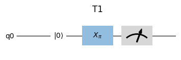
We can inspect the details of the schedule in three different ways: via (1) circuit and (2) pulse diagrams, or through (3) a timing table containing the timing and other information of each operation.
The
plot_circuit_diagram()
method can directly be used to display the quantum circuit that corresponds to
the schedule that we defined above.
t1_schedule = t1_sched(times=[1e-6])
t1_schedule.plot_circuit_diagram();

For displaying the pulse diagram and timing table, the schedule first needs to get timing information for each operation in the schedule. This is achieved by compiling the schedule using SerialCompiler. Please note that below in section 5. Experiment Execution and Analysis, the compilation is handled by MeasurementControl internally; it is done here only to enable displaying the timing table and pulse diagram.
Compiling to Hardware
More information on compilation can be found in Tutorial: Compiling to Hardware.
from quantify_scheduler import SerialCompiler
compiler = SerialCompiler(name="compiler", quantum_device=single_qubit_device)
compiled_schedule = compiler.compile(schedule=t1_schedule)
Each operation is compiled into pulses that can be viewed and inspected via the plot_pulse_diagram() method.
compiled_schedule.plot_pulse_diagram(plot_backend="plotly")
By passing the plotly backend, we made the above diagram interactive.
Lastly, the timing table can simply be accessed via the timing_table property of a schedule.
compiled_schedule.timing_table
| waveform_op_id | port | clock | abs_time | duration | is_acquisition | operation | wf_idx | operation_hash | |
|---|---|---|---|---|---|---|---|---|---|
| 0 | Reset('q0')_acq_0 | None | cl0.baseband | 0.0 ns | 200,000.0 ns | False | Reset('q0') | 0 | 8129217253941115744 |
| 1 | X(qubit='q0')_acq_0 | q0:mw | q0.01 | 200,000.0 ns | 20.0 ns | False | X(qubit='q0') | 0 | 5502904044048044573 |
| 2 | ResetClockPhase(clock='q0.ro',t0=0)_acq_0 | None | q0.ro | 201,000.0 ns | 0.0 ns | False | ResetClockPhase(clock='q0.ro',t0=0) | 0 | -4670433047108969828 |
| 3 | SquarePulse(amp=0.1,duration=4e-09,port='q0:res',clock='q0.ro',reference_magnitude=None,t0=2.96e-07)_acq_0 | q0:res | q0.ro | 201,000.0 ns | 0.0 ns | False | SquarePulse(amp=0.1,duration=4e-09,port='q0:res',clock='q0.ro',reference_magnitude=None,t0=2.96e-07) | 0 | 8748020945484081312 |
| 6 | SSBIntegrationComplex(port='q0:res',clock='q0.ro',duration=1e-06,acq_channel=0,coords=None,acq_index=None,bin_mode='average',phase=0,t0=1e-07)_acq_0 | q0:res | q0.ro | 201,100.0 ns | 1,000.0 ns | True | SSBIntegrationComplex(port='q0:res',clock='q0.ro',duration=1e-06,acq_channel=0,coords=None,acq_index=None,bin_mode='average',phase=0,t0=1e-07) | 0 | 7435596139328065232 |
| 4 | SquarePulse(amp=0.1,duration=4e-09,port='q0:res',clock='q0.ro',reference_magnitude=None,t0=2.96e-07)_acq_1 | q0:res | q0.ro | 201,296.0 ns | 0.0 ns | False | SquarePulse(amp=0.1,duration=4e-09,port='q0:res',clock='q0.ro',reference_magnitude=None,t0=2.96e-07) | 1 | 8748020945484081312 |
| 5 | SquarePulse(amp=0.1,duration=4e-09,port='q0:res',clock='q0.ro',reference_magnitude=None,t0=2.96e-07)_acq_2 | q0:res | q0.ro | 201,296.0 ns | 4.0 ns | False | SquarePulse(amp=0.1,duration=4e-09,port='q0:res',clock='q0.ro',reference_magnitude=None,t0=2.96e-07) | 2 | 8748020945484081312 |
Device-layer Schedules (Pulses)
More information on defining schedules using pulses can be found in Tutorial: Schedules and Pulses.
Circuit-layer Schedules (Gates and Measurements)
More information on defining schedules using circuit-layer operations and mixing with pulses can be found in Tutorial: Operations and Qubits.
5. Experiment Execution and Analysis#
We can now configure our MeasurementControl to run the experiment. In
this case, we will perform a 1-dimensional sweep using a
qcodes.instrument.parameter.ManualParameter. Sweeping such a parameter will physically change the hardware output as the sweep is performed.
import numpy as np
from qcodes.instrument.parameter import ManualParameter
from quantify_scheduler import ScheduleGettable
# Configure the settable
time = ManualParameter("sample", label="Sample time", unit="s")
time.batched = True
times = np.linspace(start=1.6e-7, stop=4.976e-5, num=125)
# Configure the gettable
gettable = ScheduleGettable(
quantum_device=single_qubit_device,
schedule_function=t1_sched,
schedule_kwargs={"times": times},
batched=True
)
# Configure MeasurementControl
measurement_control.settables(time)
measurement_control.setpoints(times)
measurement_control.gettables(gettable)
In the above example, we use
settables() and
gettables() together
with batched=True to instruct measurement_control how to execute the
experiment. Instead of iteratively processing each value in the times array, all are
processed in one batch.
Configuring MeasurementControl
More information on configuring MeasurementControl can be found in the
user guide
of quantify-core.
Once MeasurementControl is all set
up, we can run the experiment.
dataset = measurement_control.run()
The result of the experiment is assigned to the variable dataset, but also saved to disk (as set by set_datadir() at the start of this tutorial).
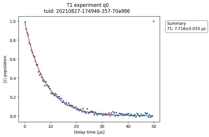
To analyze the experiment results, we can choose from the variety of classes from the quantify_core.analysis
package. For a T1 experiment, we use the
T1Analysis class which
is used to fit the data, extract relevant parameters and visualize the result.
In this tutorial, we run the experiment on a dummy cluster, and therefore the
dataset that we obtain is empty. For demonstrational purposes, we show how it
would look on an actual dataset. This example dataset can be downloaded
here.
import xarray
dataset = xarray.open_dataset("../examples/dataset.hdf5")
from quantify_core.analysis import T1Analysis
T1Analysis(dataset=dataset).run().display_figs_mpl()

Analyzing Datasets
More information on analyzing datasets can be found in the user guide
of quantify-core.