`quantify_core.analysis`#

`base_analysis`#

Module containing the analysis abstract base class and several basic analyses.

class AnalysisMeta(name, bases, namespace, /, **kwargs)[source]#

Bases: ABCMeta

Metaclass, whose purpose is to avoid storing large amount of figure in memory.

By convention, analysis object stores figures in self.figs_mpl and self.axs_mpl dictionaries. This causes troubles for long-running operations, because figures are all in memory and eventually this uses all available memory of the PC. In order to avoid it, BaseAnalysis.create_figures() and its derivatives are patched so that all the figures are put in LRU cache and reconstructed upon request to BaseAnalysis.figs_mpl or BaseAnalysis.axs_mpl if they were removed from the cache.

Provided that analyses subclasses follow convention of figures being created in BaseAnalysis.create_figures(), this approach should solve the memory issue and preserve reverse compatibility with present code.

class AnalysisSteps(value)[source]#

Bases: Enum

An enumerate of the steps executed by the BaseAnalysis (and the default for subclasses).

The involved steps are:

AnalysisSteps.STEP_1_PROCESS_DATA (BaseAnalysis.process_data())
AnalysisSteps.STEP_2_RUN_FITTING (BaseAnalysis.run_fitting())
AnalysisSteps.STEP_3_ANALYZE_FIT_RESULTS (BaseAnalysis.analyze_fit_results())
AnalysisSteps.STEP_4_CREATE_FIGURES (BaseAnalysis.create_figures())
AnalysisSteps.STEP_5_ADJUST_FIGURES (BaseAnalysis.adjust_figures())
AnalysisSteps.STEP_6_SAVE_FIGURES (BaseAnalysis.save_figures())
AnalysisSteps.STEP_7_SAVE_QUANTITIES_OF_INTEREST (BaseAnalysis.save_quantities_of_interest())
AnalysisSteps.STEP_8_SAVE_PROCESSED_DATASET (BaseAnalysis.save_processed_dataset())
AnalysisSteps.STEP_9_SAVE_FIT_RESULTS (BaseAnalysis.save_fit_results())

A custom analysis flow (e.g. inserting new steps) can be created by implementing an object similar to this one and overriding the analysis_steps.

class BaseAnalysis(dataset=None, tuid=None, label='', settings_overwrite=None, plot_figures=True)[source]#

Bases: object

A template for analysis classes.

analysis_steps#

Defines the steps of the analysis specified as an Enum. Can be overridden in a subclass in order to define a custom analysis flow. See AnalysisSteps for a template.

alias of AnalysisSteps

__init__(dataset=None, tuid=None, label='', settings_overwrite=None, plot_figures=True)[source]#

Initializes the variables used in the analysis and to which data is stored.

Warning

We highly discourage overriding the class initialization. If the analysis requires the user passing in any arguments, the run() should be overridden and extended (see its docstring for an example).

Settings schema:

Base analysis settings
properties
mpl_dpi	Matplotlib figures DPI.
	type	integer
mpl_exclude_fig_titles	If `True` maplotlib figures will not include the title.
	type	boolean
mpl_transparent_background	If `True` maplotlib figures will have transparent background (when applicable).
	type	boolean
mpl_fig_formats	List of formats in which matplotlib figures will be saved. E.g. `['svg']`
	type	array
	items	type	string

Parameters:

dataset (xr.Dataset (default: None)) – an unprocessed (raw) quantify dataset to perform the analysis on.
tuid (TUID | str (default: None)) – if no dataset is specified, will look for the dataset with the matching tuid in the data directory.
label (str (default: '')) – if no dataset and no tuid is provided, will look for the most recent dataset that contains “label” in the name.
settings_overwrite (dict (default: None)) – A dictionary containing overrides for the global base_analysis.settings for this specific instance. See Settings schema above for available settings.
plot_figures (bool (default: True)) – Option to create and save figures for analysis.

static _get_analysis_dir(tuid, name, create_missing=True)[source]#

Generate an analysis dir based on a given tuid and analysis class name.

Parameters:

tuid (TUID) – TUID of the analysis dir.
name (str) – The name of the analysis class.
create_missing (bool (default: True)) – If True, create the analysis dir if it does not already exist.

static _get_results_dir(analysis_dir, create_missing=True)[source]#

Generate an results dir based on a given analysis dir path.

Parameters:

analysis_dir (str) – The path of the analysis directory.
create_missing (bool (default: True)) – If True, create the analysis dir if it does not already exist.

adjust_clim(vmin, vmax, ax_ids=None)[source]#

Adjust the clim of matplotlib figures generated by analysis object.

Parameters:

vmin (float) – The bottom vlim in data coordinates. Passing None leaves the limit unchanged.
vmax (float) – The top vlim in data coordinates. Passing None leaves the limit unchanged.
ax_ids (Optional[list[str]] (default: None)) – A list of ax_ids specifying what axes to adjust. Passing None results in all axes of an analysis object being adjusted.

Return type:

None

adjust_cmap(cmap, ax_ids=None)[source]#

Adjust the cmap of matplotlib figures generated by analysis object.

Parameters:

cmap (Colormap | str | None) – The colormap to set for the axis
ax_ids (list[str] (default: None)) – A list of ax_ids specifying what axes to adjust. Passing None results in all axes of an analysis object being adjusted.

adjust_figures()[source]#

Perform global adjustments after creating the figures but before saving them.

By default applies mpl_exclude_fig_titles and mpl_transparent_background from .settings_overwrite to any matplotlib figures in .figs_mpl.

Can be extended in a subclass for additional adjustments.

adjust_xlim(xmin=None, xmax=None, ax_ids=None)[source]#

Adjust the xlim of matplotlib figures generated by analysis object.

Parameters:

xmin (Optional[float] (default: None)) – The bottom xlim in data coordinates. Passing None leaves the limit unchanged.
xmax (Optional[float] (default: None)) – The top xlim in data coordinates. Passing None leaves the limit unchanged.
ax_ids (Optional[list[str]] (default: None)) – A list of ax_ids specifying what axes to adjust. Passing None results in all axes of an analysis object being adjusted.

Return type:

None

adjust_ylim(ymin=None, ymax=None, ax_ids=None)[source]#

Adjust the ylim of matplotlib figures generated by analysis object.

Parameters:

ymin (Optional[float] (default: None)) – The bottom ylim in data coordinates. Passing None leaves the limit unchanged.
ymax (Optional[float] (default: None)) – The top ylim in data coordinates. Passing None leaves the limit unchanged.
ax_ids (Optional[list[str]] (default: None)) – A list of ax_ids specifying what axes to adjust. Passing None results in all axes of an analysis object being adjusted.

Return type:

None

analyze_fit_results()[source]#

To be implemented by subclasses.

Should analyze and process the .fit_results and add the quantities of interest to the .quantities_of_interest dictionary.

create_figures()[source]#

To be implemented by subclasses.

Should generate figures of interest. matplolib figures and axes objects should be added to the .figs_mpl and axs_mpl dictionaries., respectively.

display_figs_mpl()[source]#: Displays figures in .figs_mpl in all frontends.

execute_analysis_steps()[source]#

Executes the methods corresponding to the analysis steps as defined by the analysis_steps.

Intended to be called by .run when creating a custom analysis that requires passing analysis configuration arguments to run().

extract_data()[source]#

If no dataset is provided, populates .dataset with data from the experiment matching the tuid/label.

This method should be overwritten if an analysis does not relate to a single datafile.

get_flow()[source]#

Returns a tuple with the ordered methods to be called by run analysis. Only return the figures methods if self.plot_figures is True.

Return type:: tuple

classmethod load_fit_result(tuid, fit_name)[source]#

Load a saved lmfit.model.ModelResult object from file. For analyses that use custom fit functions, the cls.fit_function_definitions object must be defined in the subclass for that analysis.

Parameters:

tuid (TUID) – The TUID reference of the saved analysis.
fit_name (str) – The name of the fit result to be loaded.

Return type:

ModelResult

Returns:

: The lmfit model result object.

process_data()[source]#

To be implemented by subclasses.

Should process, e.g., reshape, filter etc. the data before starting the analysis.

run()[source]#

Execute analysis.

This function is at the core of all analysis. It calls execute_analysis_steps() which executes all the methods defined in the.

First step of any analysis is always extracting data, that is not configurable. Errors in extract_data() are considered fatal for analysis. Later steps are configurable by overriding analysis_steps. Exceptions in these steps are logged and suppressed and analysis is considered partially successful.

This function is typically called right after instantiating an analysis class.

Implementing a custom analysis that requires user input

When implementing your own custom analysis you might need to pass in a few configuration arguments. That should be achieved by overriding this function as show below.

from quantify_core.analysis.base_analysis import BaseAnalysis

class MyAnalysis(BaseAnalysis):
    def run(self, optional_argument_one: float = 3.5e9):
        # Save the value to be used in some step of the analysis
        self.optional_argument_one = optional_argument_one

        # Execute the analysis steps
        self.execute_analysis_steps()
        # Return the analysis object
        return self

    # ... other relevant methods ...

Return type:

BaseAnalysis

Returns:

: The instance of the analysis object so that run() returns an analysis object. You can initialize, run and assign it to a variable on a single line:, e.g. a_obj = MyAnalysis().run().

run_fitting()[source]#

To be implemented by subclasses.

Should create fitting model(s) and fit data to the model(s) adding the result to the .fit_results dictionary.

save_figures()[source]#

Saves figures to disk. By default saves matplotlib figures.

Can be overridden or extended to make use of other plotting packages.

save_figures_mpl(close_figs=True)[source]#

Saves all the matplotlib figures in the .figs_mpl dict.

Parameters:: close_figs (bool (default: True)) – If True, closes matplotlib figures after saving.

save_fit_results()[source]#: Saves the lmfit.model.model_result objects for each fit in a sub-directory within the analysis directory.

save_processed_dataset()[source]#: Saves a copy of the processed .dataset_processed in the analysis folder of the experiment.

save_quantities_of_interest()[source]#

Saves the .quantities_of_interest as a JSON file in the analysis directory.

The file is written using json.dump() with the qcodes.utils.NumpyJSONEncoder custom encoder.

property analysis_dir#: Analysis dir based on the tuid of the analysis class instance. Will create a directory if it does not exist.

property name#: The name of the analysis, used in data saving.

property results_dir#: Analysis dirrectory for this analysis. Will create a directory if it does not exist.

class Basic1DAnalysis(dataset=None, tuid=None, label='', settings_overwrite=None, plot_figures=True)[source]#

Bases: BasicAnalysis

Deprecated. Alias of BasicAnalysis for backwards compatibility.

run()[source]#

Execute analysis.

This function is at the core of all analysis. It calls execute_analysis_steps() which executes all the methods defined in the.

This function is typically called right after instantiating an analysis class.

Implementing a custom analysis that requires user input

When implementing your own custom analysis you might need to pass in a few configuration arguments. That should be achieved by overriding this function as show below.

from quantify_core.analysis.base_analysis import BaseAnalysis

class MyAnalysis(BaseAnalysis):
    def run(self, optional_argument_one: float = 3.5e9):
        # Save the value to be used in some step of the analysis
        self.optional_argument_one = optional_argument_one

        # Execute the analysis steps
        self.execute_analysis_steps()
        # Return the analysis object
        return self

    # ... other relevant methods ...

Return type:

BaseAnalysis

Returns:

: The instance of the analysis object so that run() returns an analysis object. You can initialize, run and assign it to a variable on a single line:, e.g. a_obj = MyAnalysis().run().

class Basic2DAnalysis(dataset=None, tuid=None, label='', settings_overwrite=None, plot_figures=True)[source]#

Bases: BaseAnalysis

A basic analysis that extracts the data from the latest file matching the label and plots and stores the data in the experiment container.

create_figures()[source]#

To be implemented by subclasses.

Should generate figures of interest. matplolib figures and axes objects should be added to the .figs_mpl and axs_mpl dictionaries., respectively.

class BasicAnalysis(dataset=None, tuid=None, label='', settings_overwrite=None, plot_figures=True)[source]#

Bases: BaseAnalysis

A basic analysis that extracts the data from the latest file matching the label and plots and stores the data in the experiment container.

create_figures()[source]#: Creates a line plot x vs y for every data variable yi and coordinate xi in the dataset.

class _FiguresMplCache(figs, axes, initialized)[source]#: Bases: object

analysis_steps_to_str(analysis_steps, class_name='BaseAnalysis')[source]#

A utility for generating the docstring for the analysis steps.

Parameters:

analysis_steps (Enum) – An Enum similar to quantify_core.analysis.base_analysis.AnalysisSteps.
class_name (str (default: 'BaseAnalysis')) – The class name that has the analysis_steps methods and for which the analysis_steps are intended.

Return type:

str

Returns:

: A formatted string version of the analysis_steps and corresponding methods.

check_lmfit(fit_res)[source]#

Check that lmfit was able to successfully return a valid fit, and give a warning if not.

The function looks at lmfit’s success parameter, and also checks whether the fit was able to obtain valid error bars on the fitted parameters.

Parameters:

fit_res (ModelResult) – The ModelResult object output by lmfit

Return type:

str

Returns:

: A warning message if there is a problem with the fit.

flatten_lmfit_modelresult(model)[source]#

Flatten an lmfit model result to a dictionary in order to be able to save it to disk.

Notes

We use this method as opposed to save_modelresult() as the corresponding load_modelresult() cannot handle loading data with a custom fit function.

lmfit_par_to_ufloat(param)[source]#

Safe conversion of an lmfit.parameter.Parameter to uncertainties.ufloat(value, std_dev).

This function is intended to be used in custom analyses to avoid errors when an lmfit fails and the stderr is None.

Parameters:: param (Parameter) – The Parameter to be converted
Returns:: uncertainties.UFloat : An object representing the value and the uncertainty of the parameter.

wrap_text(text, width=35, replace_whitespace=True, **kwargs)[source]#

A text wrapping (braking over multiple lines) utility.

Intended to be used with plot_textbox() in order to avoid too wide figure when, e.g., check_lmfit() fails and a warning message is generated.

For usage see, for example, source code of create_figures().

Parameters:

text – The text string to be wrapped over several lines.
width (default: 35) – Maximum line width in characters.
replace_whitespace (default: True) – Passed to textwrap.wrap() and documented here.
kwargs – Any other keyword arguments to be passed to textwrap.wrap().

Returns:

: The wrapped text (or None if text is None).

settings = {'mpl_dpi': 450, 'mpl_fig_formats': ['png', 'svg'], 'mpl_exclude_fig_titles': False, 'mpl_transparent_background': True}#

For convenience the analysis framework provides a set of global settings.

For available settings see BaseAnalysis. These can be overwritten for each instance of an analysis.

Examples

>>> from quantify_core.analysis import base_analysis as ba
... ba.settings["mpl_dpi"] = 300  # set resolution of matplotlib figures

`cosine_analysis`#

Module containing an education example of an analysis subclass.

See Tutorial 3. Building custom analyses - the data analysis framework that guides you through the process of building this analysis.

class CosineAnalysis(dataset=None, tuid=None, label='', settings_overwrite=None, plot_figures=True)[source]#

Bases: BaseAnalysis

Exemplary analysis subclass that fits a cosine to a dataset.

analyze_fit_results()[source]#: Checks fit success and populates quantities_of_interest.

create_figures()[source]#: Creates a figure with the data and the fit.

process_data()[source]#

In some cases, you might need to process the data, e.g., reshape, filter etc., before starting the analysis. This is the method where it should be done.

See process_data() for an implementation example.

run_fitting()[source]#: Fits a CosineModel to the data.

`spectroscopy_analysis`#

class QubitFluxSpectroscopyAnalysis(dataset=None, tuid=None, label='', settings_overwrite=None, plot_figures=True)[source]#

Bases: BaseAnalysis

Analysis class for qubit flux spectroscopy.

Example

from quantify_core.analysis.spectroscopy_analysis import QubitFluxSpectroscopyAnalysis
import quantify_core.data.handling as dh

# load example data
test_data_dir = "../tests/test_data"
dh.set_datadir(test_data_dir)

# run analysis and plot results
analysis = (
    QubitFluxSpectroscopyAnalysis(tuid="20230309-235354-353-9c94c5")
    .run()
    .display_figs_mpl()
)

analyze_fit_results()[source]#

Check the fit success and populate .quantities_of_interest.

Return type:: None

create_figures()[source]#

Generate plot of magnitude and phase images, with superposed model fit.

Return type:: None

process_data()[source]#

Process the data so that the analysis can make assumptions on the format.

Return type:: None

run_fitting()[source]#

Fits a QuadraticModel model to the frequency response vs. flux offset.

Return type:: None

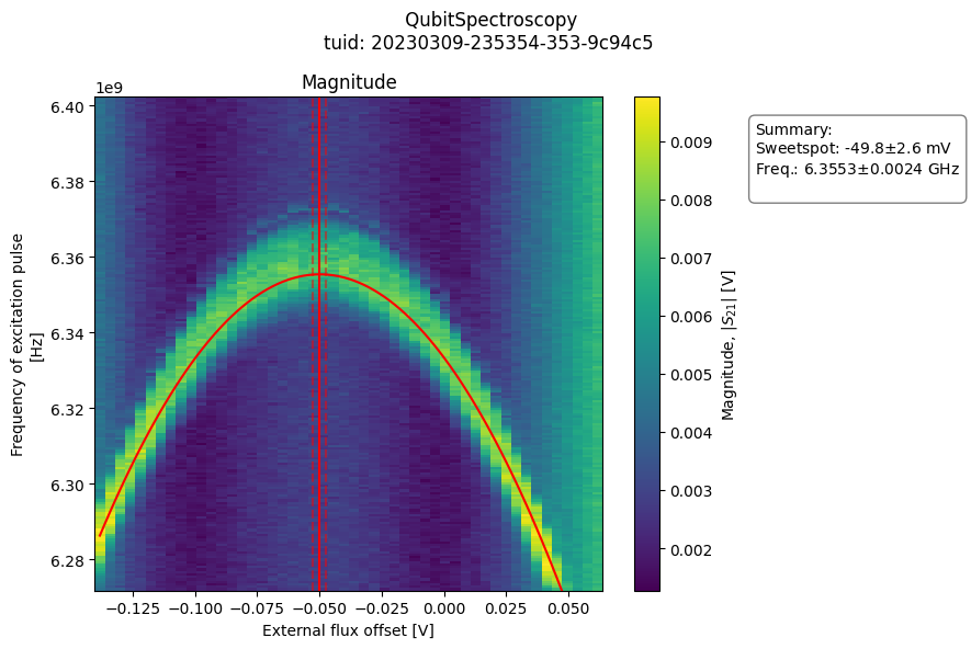
class QubitSpectroscopyAnalysis(dataset=None, tuid=None, label='', settings_overwrite=None, plot_figures=True)[source]#

Bases: BaseAnalysis

Analysis for a qubit spectroscopy experiment.

Fits a Lorentzian function to qubit spectroscopy data and finds the 0-1 transistion frequency.

analyze_fit_results()[source]#

Check fit success and populates .quantities_of_interest.

Return type:: None

create_figures()[source]#

Create qubit spectroscopy figure.

Return type:: None

process_data()[source]#

Populate the .dataset_processed.

Return type:: None

run_fitting()[source]#

Fit a Lorentzian function to the data.

Return type:: None

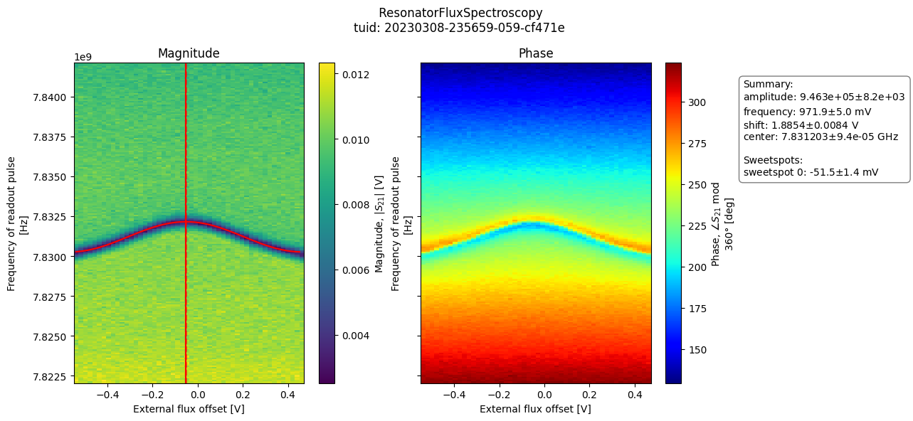
class ResonatorFluxSpectroscopyAnalysis(dataset=None, tuid=None, label='', settings_overwrite=None, plot_figures=True)[source]#

Bases: BaseAnalysis

Analysis class for resonator flux spectroscopy.

Example

from quantify_core.analysis.spectroscopy_analysis import (
    ResonatorFluxSpectroscopyAnalysis
)
import quantify_core.data.handling as dh

# load example data
test_data_dir = "../tests/test_data"
dh.set_datadir(test_data_dir)

# run analysis and plot results
analysis = (
    ResonatorFluxSpectroscopyAnalysis(tuid="20230308-235659-059-cf471e")
    .run()
    .display_figs_mpl()
)

analyze_fit_results()[source]#

Check the fit success and populate .quantities_of_interest.

Return type:: None

create_figures()[source]#

Generate plot of magnitude and phase images, with superposed model fit.

Return type:: None

process_data()[source]#

Process the data so that the analysis can make assumptions on the format.

Return type:: None

run_fitting()[source]#

Fits a sinusoidal model to the frequency response vs. flux offset.

Return type:: None

class ResonatorSpectroscopyAnalysis(dataset=None, tuid=None, label='', settings_overwrite=None, plot_figures=True)[source]#

Bases: BaseAnalysis

Analysis for a spectroscopy experiment of a hanger resonator.

analyze_fit_results()[source]#: Checks fit success and populates .quantities_of_interest.

create_figures()[source]#: Plots the measured and fitted transmission \(S_{21}\) as the I and Q component vs frequency, the magnitude and phase vs frequency, and on the complex I,Q plane.

process_data()[source]#: Verifies that the data is measured as magnitude and phase and casts it to a dataset of complex valued transmission \(S_{21}\).

run_fitting()[source]#: Fits a ResonatorModel to the data.

`single_qubit_timedomain`#

Module containing analyses for common single qubit timedomain experiments.

class AllXYAnalysis(dataset=None, tuid=None, label='', settings_overwrite=None, plot_figures=True)[source]#

Bases: SingleQubitTimedomainAnalysis

Normalizes the data from an AllXY experiment and plots against an ideal curve.

See section 2.3.2 of Reed [2013] for an explanation of the AllXY experiment and it’s applications in diagnosing errors in single-qubit control pulses.

create_figures()[source]#

To be implemented by subclasses.

Should generate figures of interest. matplolib figures and axes objects should be added to the .figs_mpl and axs_mpl dictionaries., respectively.

process_data()[source]#

Processes the data so that the analysis can make assumptions on the format.

Populates self.dataset_processed.S21 with the complex (I,Q) valued transmission, and if calibration points are present for the 0 and 1 state, populates self.dataset_processed.pop_exc with the excited state population.

run()[source]#

Executes the analysis using specific datapoints as calibration points.

Returns:: AllXYAnalysis: The instance of this analysis.

class EchoAnalysis(dataset=None, tuid=None, label='', settings_overwrite=None, plot_figures=True)[source]#

Bases: SingleQubitTimedomainAnalysis, _DecayFigMixin

Analysis class for a qubit spin-echo experiment, which fits an exponential decay and extracts the T2_echo time.

analyze_fit_results()[source]#: Checks fit success and populates .quantities_of_interest.

create_figures()[source]#: Create a figure showing the exponential decay and fit.

run_fitting()[source]#: Fit the data to ExpDecayModel.

class RabiAnalysis(dataset=None, tuid=None, label='', settings_overwrite=None, plot_figures=True)[source]#

Bases: SingleQubitTimedomainAnalysis

Fits a cosine curve to Rabi oscillation data and finds the qubit drive amplitude required to implement a pi-pulse.

The analysis will automatically rotate the data so that the data lies along the axis with the best SNR.

_rotate_to_calibrated_axis()[source]#

If calibration points are True, automatically determine the point farthest from the 0 point to use as a reference to rotate the data.

This will ensure the data lies along the axis with the best SNR.

analyze_fit_results()[source]#: Checks fit success and populates .quantities_of_interest.

create_figures()[source]#: Creates Rabi oscillation figure

run(calibration_points=True)[source]#

Parameters:: calibration_points (bool (default: True)) – Specifies if the data should be rotated so that it lies along the axis with the best SNR.
Returns:: RabiAnalysis: The instance of this analysis.

run_fitting()[source]#: Fits a RabiModel to the data.

class RamseyAnalysis(dataset=None, tuid=None, label='', settings_overwrite=None, plot_figures=True)[source]#

Bases: SingleQubitTimedomainAnalysis, _DecayFigMixin

Fits a decaying cosine curve to Ramsey data (possibly with artificial detuning) and finds the true detuning, qubit frequency and T2* time.

analyze_fit_results()[source]#: Extract the real detuning and qubit frequency based on the artificial detuning and fitted detuning.

create_figures()[source]#: Plot Ramsey decay figure.

run(artificial_detuning=0, qubit_frequency=None, calibration_points='auto')[source]#

Parameters:

artificial_detuning (float (default: 0)) – The detuning in Hz that will be emulated by adding an extra phase in software.
qubit_frequency (Optional[float] (default: None)) – The initial recorded value of the qubit frequency (before accurate fitting is done) in Hz.
calibration_points (Union[bool, Literal['auto']] (default: 'auto')) – Indicates if the data analyzed includes calibration points. If set to True, will interpret the last two data points in the dataset as \(|0\rangle\) and \(|1\rangle\) respectively. If "auto", will use has_calibration_points() to determine if the data contains calibration points.

Returns:

RamseyAnalysis: The instance of this analysis.

run_fitting()[source]#: Fits a DecayOscillationModel to the data.

class SingleQubitTimedomainAnalysis(dataset=None, tuid=None, label='', settings_overwrite=None, plot_figures=True)[source]#

Bases: BaseAnalysis

Base Analysis class for single-qubit timedomain experiments.

process_data()[source]#

Processes the data so that the analysis can make assumptions on the format.

run(calibration_points='auto')[source]#

Parameters:: calibration_points (Union[bool, Literal['auto']] (default: 'auto')) – Indicates if the data analyzed includes calibration points. If set to True, will interpret the last two data points in the dataset as \(|0\rangle\) and \(|1\rangle\) respectively. If "auto", will use has_calibration_points() to determine if the data contains calibration points.
Returns:: SingleQubitTimedomainAnalysis: The instance of this analysis.

class T1Analysis(dataset=None, tuid=None, label='', settings_overwrite=None, plot_figures=True)[source]#

Bases: SingleQubitTimedomainAnalysis, _DecayFigMixin

Analysis class for a qubit T1 experiment, which fits an exponential decay and extracts the T1 time.

analyze_fit_results()[source]#: Checks fit success and populates .quantities_of_interest.

create_figures()[source]#: Create a figure showing the exponential decay and fit.

run_fitting()[source]#: Fit the data to ExpDecayModel.

class _DecayFigMixin[source]#

Bases: object

A mixin for common analysis logic.

_create_decay_figure(fig_id)[source]#: Creates a figure ready for plotting a fit.

`interpolation_analysis`#

class InterpolationAnalysis2D(dataset=None, tuid=None, label='', settings_overwrite=None, plot_figures=True)[source]#

Bases: BaseAnalysis

An analysis class which generates a 2D interpolating plot for each yi variable in the dataset.

create_figures()[source]#: Create a 2D interpolating figure for each yi.

`optimization_analysis`#

class OptimizationAnalysis(dataset=None, tuid=None, label='', settings_overwrite=None, plot_figures=True)[source]#

Bases: BaseAnalysis

An analysis class which extracts the optimal quantities from an N-dimensional interpolating experiment.

create_figures()[source]#: Plot each of the x variables against each of the y variables.

process_data()[source]#: Finds the optimal (minimum or maximum) for y0 and saves the xi and y0 values in the quantities_of_interest.

run(minimize=True)[source]#

Parameters:: minimize (bool (default: True)) – Boolean which determines whether to report the minimum or the maximum. True for minimize. False for maximize.
Returns:: OptimizationAnalysis: The instance of this analysis.

iteration_plots(dataset, quantities_of_interest)[source]#: For every x and y variable, plot a graph of that variable vs the iteration index.

`fitting_models`#

Models and fit functions to be used with the lmfit fitting framework.

class CosineModel(*args, **kwargs)[source]#

Bases: Model

Exemplary lmfit model with a guess for a cosine.

Note

The lmfit.models module provides several fitting models that might fit your needs out of the box.

__init__(*args, **kwargs)[source]#

Parameters:

independent_vars (list of str) – Arguments to the model function that are independent variables default is ['x']).
prefix (str) – String to prepend to parameter names, needed to add two Models that have parameter names in common.
nan_policy – How to handle NaN and missing values in data. See Notes below.
**kwargs – Keyword arguments to pass to Model.

Notes

1. nan_policy sets what to do when a NaN or missing value is seen in the data. Should be one of:

‘raise’ : raise a ValueError (default)

‘propagate’ : do nothing

‘omit’ : drop missing data

See also

cos_func()

guess(data, x, **kws)[source]#

Guess starting values for the parameters of a model.

Parameters:

data (ndarray) – Array of data (i.e., y-values) to use to guess parameter values.
x (ndarray) – Array of values for the independent variable (i.e., x-values).
**kws – Additional keyword arguments, passed to model function.

Return type:

Parameters

Returns:

paramsParameters: Initial, guessed values for the parameters of a Model.

Changed in version 1.0.3: Argument x is now explicitly required to estimate starting values.

class DecayOscillationModel(*args, **kwargs)[source]#

Bases: Model

Model for a decaying oscillation which decays to a point with 0 offset from the centre of the of the oscillation (as in a Ramsey experiment, for example).

__init__(*args, **kwargs)[source]#

Parameters:

independent_vars (list of str) – Arguments to the model function that are independent variables default is ['x']).
prefix (str) – String to prepend to parameter names, needed to add two Models that have parameter names in common.
nan_policy – How to handle NaN and missing values in data. See Notes below.
**kwargs – Keyword arguments to pass to Model.

Notes

1. nan_policy sets what to do when a NaN or missing value is seen in the data. Should be one of:

‘raise’ : raise a ValueError (default)

‘propagate’ : do nothing

‘omit’ : drop missing data

See also

exp_damp_osc_func()

guess(data, **kws)[source]#

Guess starting values for the parameters of a model.

Parameters:

data (ndarray) – Array of data (i.e., y-values) to use to guess parameter values.
x (ndarray) – Array of values for the independent variable (i.e., x-values).
**kws – Additional keyword arguments, passed to model function.

Return type:

Parameters

Returns:

paramsParameters: Initial, guessed values for the parameters of a Model.

Changed in version 1.0.3: Argument x is now explicitly required to estimate starting values.

class ExpDecayModel(*args, **kwargs)[source]#

Bases: Model

Model for an exponential decay, such as a qubit T1 measurement.

__init__(*args, **kwargs)[source]#

Parameters:

independent_vars (list of str) – Arguments to the model function that are independent variables default is ['x']).
prefix (str) – String to prepend to parameter names, needed to add two Models that have parameter names in common.
nan_policy – How to handle NaN and missing values in data. See Notes below.
**kwargs – Keyword arguments to pass to Model.

Notes

1. nan_policy sets what to do when a NaN or missing value is seen in the data. Should be one of:

‘raise’ : raise a ValueError (default)

‘propagate’ : do nothing

‘omit’ : drop missing data

See also

exp_decay_func()

guess(data, **kws)[source]#

Guess starting values for the parameters of a model.

Parameters:

data (ndarray) – Array of data (i.e., y-values) to use to guess parameter values.
x (ndarray) – Array of values for the independent variable (i.e., x-values).
**kws – Additional keyword arguments, passed to model function.

Return type:

Parameters

Returns:

paramsParameters: Initial, guessed values for the parameters of a Model.

Changed in version 1.0.3: Argument x is now explicitly required to estimate starting values.

class LorentzianModel(*args, **kwargs)[source]#

Bases: Model

Model for data which follows a Lorentzian function.

Uses the function lorentzian_func() as the defining equation.

guess(data, **kws)[source]#

Guess some initial values for the model based on the data.

Return type:: Parameters

class RabiModel(*args, **kwargs)[source]#

Bases: Model

Model for a Rabi oscillation as a function of the microwave drive amplitude. Phase of oscillation is fixed at \(\pi\) in order to ensure that the oscillation is at a minimum when the drive amplitude is 0.

__init__(*args, **kwargs)[source]#

Parameters:

independent_vars (list of str) – Arguments to the model function that are independent variables default is ['x']).
prefix (str) – String to prepend to parameter names, needed to add two Models that have parameter names in common.
nan_policy – How to handle NaN and missing values in data. See Notes below.
**kwargs – Keyword arguments to pass to Model.

Notes

1. nan_policy sets what to do when a NaN or missing value is seen in the data. Should be one of:

‘raise’ : raise a ValueError (default)

‘propagate’ : do nothing

‘omit’ : drop missing data

See also

cos_func()

guess(data, **kws)[source]#

Guess starting values for the parameters of a model.

Parameters:

data (ndarray) – Array of data (i.e., y-values) to use to guess parameter values.
x (ndarray) – Array of values for the independent variable (i.e., x-values).
**kws – Additional keyword arguments, passed to model function.

Return type:

Parameters

Returns:

paramsParameters: Initial, guessed values for the parameters of a Model.

Changed in version 1.0.3: Argument x is now explicitly required to estimate starting values.

class ResonatorModel(*args, **kwargs)[source]#

Bases: Model

Resonator model

Implementation and design patterns inspired by the complex resonator model example (lmfit documentation).

__init__(*args, **kwargs)[source]#

Parameters:

independent_vars (list of str) – Arguments to the model function that are independent variables default is ['x']).
prefix (str) – String to prepend to parameter names, needed to add two Models that have parameter names in common.
nan_policy – How to handle NaN and missing values in data. See Notes below.
**kwargs – Keyword arguments to pass to Model.

Notes

1. nan_policy sets what to do when a NaN or missing value is seen in the data. Should be one of:

‘raise’ : raise a ValueError (default)

‘propagate’ : do nothing

‘omit’ : drop missing data

See also

hanger_func_complex_SI()

guess(data, **kws)[source]#

Guess starting values for the parameters of a model.

Parameters:

data (ndarray) – Array of data (i.e., y-values) to use to guess parameter values.
x (ndarray) – Array of values for the independent variable (i.e., x-values).
**kws – Additional keyword arguments, passed to model function.

Return type:

Parameters

Returns:

paramsParameters: Initial, guessed values for the parameters of a Model.

Changed in version 1.0.3: Argument x is now explicitly required to estimate starting values.

cos_func(x, frequency, amplitude, offset, phase=0)[source]#

An oscillating cosine function:

\(y = \mathrm{amplitude} \times \cos(2 \pi \times \mathrm{frequency} \times x + \mathrm{phase}) + \mathrm{offset}\)

Parameters:

x (float) – The independent variable (time, for example)
frequency (float) – A generalized frequency (in units of inverse x)
amplitude (float) – Amplitude of the oscillation
offset (float) – Output signal vertical offset
phase (float (default: 0)) – Phase offset / rad

Return type:

float

Returns:

: Output signal magnitude

exp_damp_osc_func(t, tau, n_factor, frequency, phase, amplitude, offset)[source]#

A sinusoidal oscillation with an exponentially decaying envelope function:

\(y = \mathrm{amplitude} \times \exp\left(-(t/\tau)^\mathrm{n\_factor}\right)(\cos(2\pi\mathrm{frequency}\times t + \mathrm{phase}) + \mathrm{oscillation_offset}) + \mathrm{exponential_offset}\)

Parameters:

t (float) – time
tau (float) – decay time
n_factor (float) – exponential decay factor
frequency (float) – frequency of the oscillation
phase (float) – phase of the oscillation
amplitude (float) – initial amplitude of the oscillation
oscillation_offset – vertical offset of cosine oscillation relative to exponential asymptote
exponential_offset – offset of exponential asymptote

Returns:

: Output of decaying cosine function as a float

exp_decay_func(t, tau, amplitude, offset, n_factor)[source]#

This is a general exponential decay function:

\(y = \mathrm{amplitude} \times \exp\left(-(t/\tau)^\mathrm{n\_factor}\right) + \mathrm{offset}\)

Parameters:

t (float) – time
tau (float) – decay time
amplitude (float) – amplitude of the exponential decay
offset (float) – asymptote of the exponential decay, the value at t=infinity
n_factor (float) – exponential decay factor

Return type:

float

Returns:

: Output of exponential function as a float

fft_freq_phase_guess(data, t)[source]#

Guess for a cosine fit using FFT, only works for evenly spaced points.

Parameters:

data (ndarray) – Input data to FFT
t (ndarray) – Independent variable (e.g. time)

Return type:

Tuple[float, float]

Returns:

freq_guess:: Guess for the frequency of the cosine function
ph_guess:: Guess for the phase of the cosine function

get_guess_common_doc()[source]#

Returns a common docstring to be used for the guess() method of custom fitting Model s. :rtype: str

Usage example for a custom fitting model

See the usage example at the end of the ResonatorModel source-code:

class ResonatorModel(lmfit.model.Model):
    """
    Resonator model

    Implementation and design patterns inspired by the
    `complex resonator model example <https://lmfit.github.io/lmfit-py/examples/example_complex_resonator_model.html>`_
    (`lmfit` documentation).

    """  # pylint: disable=line-too-long

    # pylint: disable=empty-docstring
    # pylint: disable=abstract-method
    def __init__(self, *args, **kwargs):
        # pass in the defining equation so the user doesn't have to later.
        super().__init__(hanger_func_complex_SI, *args, **kwargs)
        self.set_param_hint("Ql", min=0)  # Enforce Q is positive
        self.set_param_hint("Qe", min=0)  # Enforce Q is positive

        # Internal and coupled quality factor can be derived from fitted params
        self.set_param_hint("Qi", expr="1./(1./Ql-1./Qe*cos(theta))", vary=False)
        self.set_param_hint("Qc", expr="Qe/cos(theta)", vary=False)

    # pylint: disable=too-many-locals
    # pylint: disable=missing-function-docstring
    def guess(self, data, **kws) -> lmfit.parameter.Parameters:
        f = kws.get("f", None)
        if f is None:
            return None

        argmin_s21 = np.abs(data).argmin()
        fmin = f.min()
        fmax = f.max()
        # guess that the resonance is the lowest point
        fr_guess = f[argmin_s21]
        # assume the user isn't trying to fit just a small part of a resonance curve.
        Q_min = 0.1 * (fr_guess / (fmax - fmin))
        delta_f = np.diff(f)  # assume f is sorted
        min_delta_f = delta_f[delta_f > 0].min()
        Q_max = (
            fr_guess / min_delta_f
        )  # assume data actually samples the resonance reasonably
        Q_guess = np.sqrt(Q_min * Q_max)  # geometric mean, why not?
        (phi_0_guess, phi_v_guess) = resonator_phase_guess(
            data, f
        )  # Come up with a guess for phase velocity

        self.set_param_hint("fr", value=fr_guess, min=fmin, max=fmax)
        self.set_param_hint("Ql", value=Q_guess * 1.01, min=Q_min, max=Q_max)
        self.set_param_hint("Qe", value=Q_guess * 0.99, min=0)
        self.set_param_hint("A", value=np.mean(abs(data)), min=0)

        # The parameters below need a proper guess.
        self.set_param_hint("theta", value=0, min=-np.pi / 2, max=np.pi / 2)
        self.set_param_hint("phi_0", value=phi_0_guess)
        self.set_param_hint("phi_v", value=phi_v_guess)
        self.set_param_hint("alpha", value=0, min=-1, max=1)

        params = self.make_params()
        return lmfit.models.update_param_vals(params, self.prefix, **kws)

    # Same design patter is used in lmfit.models
    __init__.__doc__ = get_model_common_doc() + mk_seealso("hanger_func_complex_SI")
    guess.__doc__ = get_guess_common_doc()

get_model_common_doc()[source]#

Returns a common docstring to be used with custom fitting Model s. :rtype: str

Usage example for a custom fitting model

See the usage example at the end of the ResonatorModel source-code:

class ResonatorModel(lmfit.model.Model):
    """
    Resonator model

    Implementation and design patterns inspired by the
    `complex resonator model example <https://lmfit.github.io/lmfit-py/examples/example_complex_resonator_model.html>`_
    (`lmfit` documentation).

    """  # pylint: disable=line-too-long

    # pylint: disable=empty-docstring
    # pylint: disable=abstract-method
    def __init__(self, *args, **kwargs):
        # pass in the defining equation so the user doesn't have to later.
        super().__init__(hanger_func_complex_SI, *args, **kwargs)
        self.set_param_hint("Ql", min=0)  # Enforce Q is positive
        self.set_param_hint("Qe", min=0)  # Enforce Q is positive

        # Internal and coupled quality factor can be derived from fitted params
        self.set_param_hint("Qi", expr="1./(1./Ql-1./Qe*cos(theta))", vary=False)
        self.set_param_hint("Qc", expr="Qe/cos(theta)", vary=False)

    # pylint: disable=too-many-locals
    # pylint: disable=missing-function-docstring
    def guess(self, data, **kws) -> lmfit.parameter.Parameters:
        f = kws.get("f", None)
        if f is None:
            return None

        argmin_s21 = np.abs(data).argmin()
        fmin = f.min()
        fmax = f.max()
        # guess that the resonance is the lowest point
        fr_guess = f[argmin_s21]
        # assume the user isn't trying to fit just a small part of a resonance curve.
        Q_min = 0.1 * (fr_guess / (fmax - fmin))
        delta_f = np.diff(f)  # assume f is sorted
        min_delta_f = delta_f[delta_f > 0].min()
        Q_max = (
            fr_guess / min_delta_f
        )  # assume data actually samples the resonance reasonably
        Q_guess = np.sqrt(Q_min * Q_max)  # geometric mean, why not?
        (phi_0_guess, phi_v_guess) = resonator_phase_guess(
            data, f
        )  # Come up with a guess for phase velocity

        self.set_param_hint("fr", value=fr_guess, min=fmin, max=fmax)
        self.set_param_hint("Ql", value=Q_guess * 1.01, min=Q_min, max=Q_max)
        self.set_param_hint("Qe", value=Q_guess * 0.99, min=0)
        self.set_param_hint("A", value=np.mean(abs(data)), min=0)

        # The parameters below need a proper guess.
        self.set_param_hint("theta", value=0, min=-np.pi / 2, max=np.pi / 2)
        self.set_param_hint("phi_0", value=phi_0_guess)
        self.set_param_hint("phi_v", value=phi_v_guess)
        self.set_param_hint("alpha", value=0, min=-1, max=1)

        params = self.make_params()
        return lmfit.models.update_param_vals(params, self.prefix, **kws)

    # Same design patter is used in lmfit.models
    __init__.__doc__ = get_model_common_doc() + mk_seealso("hanger_func_complex_SI")
    guess.__doc__ = get_guess_common_doc()

hanger_func_complex_SI(f, fr, Ql, Qe, A, theta, phi_v, phi_0, alpha=1)[source]#

This is the complex function for a hanger (lambda/4 resonator).

Parameters:

f (float) – frequency
fr (float) – resonance frequency
A (float) – background transmission amplitude
Ql (float) – loaded quality factor of the resonator
Qe (float) – magnitude of extrinsic quality factor Qe = |Q_extrinsic|
theta (float) – phase of extrinsic quality factor (in rad)
phi_v (float) – phase to account for propagation delay to sample
phi_0 (float) – phase to account for propagation delay from sample
alpha (float (default: 1)) – slope of signal around the resonance

Return type:

complex

Returns:

: complex valued transmission

See eq. S4 from Bruno et al. (2015) ArXiv:1502.04082.

\[S_{21} = A \left(1+\alpha \frac{f-f_r}{f_r} \right) \left(1- \frac{\frac{Q_l}{|Q_e|}e^{i\theta} }{1+2iQ_l \frac{f-f_r}{f_r}} \right) e^{i (\phi_v f + \phi_0)}\]

The loaded and extrinsic quality factors are related to the internal and coupled Q according to:

\[\frac{1}{Q_l} = \frac{1}{Q_c}+\frac{1}{Q_i}\]

and

\[\frac{1}{Q_c} = \mathrm{Re}\left(\frac{1}{|Q_e|e^{-i\theta}}\right)\]

lorentzian_func(x, x0, width, a, c)[source]#

A Lorentzian function.

\[y = \frac{a*\mathrm{width}}{\pi(\mathrm{width}^2 + (x - x_0)^2)} + c\]

Parameters:

x (float) – independent variable
x0 (float) – horizontal offset
width (float) – Lorenztian linewidth
a (float) – amplitude
c (float) – vertical offset

Return type:

float

Returns:

: Lorentzian function

mk_seealso(function_name, role='func', prefix='\\n\\n', module_location='.')[source]#

Returns a sphinx seealso pointing to a function.

Intended to be used for building custom fitting model docstrings.

Usage example for a custom fitting model

See the usage example at the end of the ResonatorModel source-code:

class ResonatorModel(lmfit.model.Model):
    """
    Resonator model

    Implementation and design patterns inspired by the
    `complex resonator model example <https://lmfit.github.io/lmfit-py/examples/example_complex_resonator_model.html>`_
    (`lmfit` documentation).

    """  # pylint: disable=line-too-long

    # pylint: disable=empty-docstring
    # pylint: disable=abstract-method
    def __init__(self, *args, **kwargs):
        # pass in the defining equation so the user doesn't have to later.
        super().__init__(hanger_func_complex_SI, *args, **kwargs)
        self.set_param_hint("Ql", min=0)  # Enforce Q is positive
        self.set_param_hint("Qe", min=0)  # Enforce Q is positive

        # Internal and coupled quality factor can be derived from fitted params
        self.set_param_hint("Qi", expr="1./(1./Ql-1./Qe*cos(theta))", vary=False)
        self.set_param_hint("Qc", expr="Qe/cos(theta)", vary=False)

    # pylint: disable=too-many-locals
    # pylint: disable=missing-function-docstring
    def guess(self, data, **kws) -> lmfit.parameter.Parameters:
        f = kws.get("f", None)
        if f is None:
            return None

        argmin_s21 = np.abs(data).argmin()
        fmin = f.min()
        fmax = f.max()
        # guess that the resonance is the lowest point
        fr_guess = f[argmin_s21]
        # assume the user isn't trying to fit just a small part of a resonance curve.
        Q_min = 0.1 * (fr_guess / (fmax - fmin))
        delta_f = np.diff(f)  # assume f is sorted
        min_delta_f = delta_f[delta_f > 0].min()
        Q_max = (
            fr_guess / min_delta_f
        )  # assume data actually samples the resonance reasonably
        Q_guess = np.sqrt(Q_min * Q_max)  # geometric mean, why not?
        (phi_0_guess, phi_v_guess) = resonator_phase_guess(
            data, f
        )  # Come up with a guess for phase velocity

        self.set_param_hint("fr", value=fr_guess, min=fmin, max=fmax)
        self.set_param_hint("Ql", value=Q_guess * 1.01, min=Q_min, max=Q_max)
        self.set_param_hint("Qe", value=Q_guess * 0.99, min=0)
        self.set_param_hint("A", value=np.mean(abs(data)), min=0)

        # The parameters below need a proper guess.
        self.set_param_hint("theta", value=0, min=-np.pi / 2, max=np.pi / 2)
        self.set_param_hint("phi_0", value=phi_0_guess)
        self.set_param_hint("phi_v", value=phi_v_guess)
        self.set_param_hint("alpha", value=0, min=-1, max=1)

        params = self.make_params()
        return lmfit.models.update_param_vals(params, self.prefix, **kws)

    # Same design patter is used in lmfit.models
    __init__.__doc__ = get_model_common_doc() + mk_seealso("hanger_func_complex_SI")
    guess.__doc__ = get_guess_common_doc()

Parameters:

function_name (str) – name of the function to point to
role (str (default: 'func')) – a sphinx role, e.g. "func"
prefix (str (default: '\\n\\n')) – string preceding the seealso
module_location (str (default: '.')) – can be used to indicate a function outside this module, e.g., my_module.submodule which contains the function.

Return type:

str

Returns:

: resulting string

resonator_phase_guess(s21, freq)[source]#

Guesses the phase velocity in resonator spectroscopy, based on the median of all the differences between consecutive phases.

Parameters:

s21 (ndarray) – Resonator S21 data
freq (ndarray) – Frequency of the spectroscopy pulse

Return type:

Tuple[float, float]

Returns:

phi_0:: Guess for the phase offset
phi_v:: Guess for the phase velocity

`calibration`#

Module containing analysis utilities for calibration procedures.

In particular, manipulation of data and calibration points for qubit readout calibration.

has_calibration_points(s21, indices_state_0=(-2,), indices_state_1=(-1,))[source]#

Determine if dataset with S21 data has calibration points for 0 and 1 states.

Three pieces of information are used to infer the presence of calibration points:

The angle of the calibration points with respect to the average of the datapoints,
The distance between the calibration points, and
The average distance to the line defined be the calibration points.

The detection is made robust by averaging 3 datapoints for each extremity of the “segment” described by the data on the IQ-plane.

See also

Calibration points autodetection

Parameters:

s21 (ndarray) – Array of complex datapoints corresponding to the experiment on the IQ plane.
indices_state_0 (tuple (default: (-2,))) – Indices in the s21 array that correspond to the ground state.
indices_state_1 (tuple (default: (-1,))) – Indices in the s21 array that correspond to the first excited state.

Return type:

bool

Returns:

: The inferred presence of calibration points.

rotate_to_calibrated_axis(data, ref_val_0, ref_val_1)[source]#

Rotates, normalizes and offsets complex valued data based on calibration points.

Parameters:

data (ndarray) – An array of complex valued data points.
ref_val_0 (complex) – The reference value corresponding to the 0 state.
ref_val_1 (complex) – The reference value corresponding to the 1 state.

Return type:

ndarray

Returns:

: Calibrated array of complex data points.

`readout_calibration_analysis`#

Module containing an analysis class for two-state readout calibration.

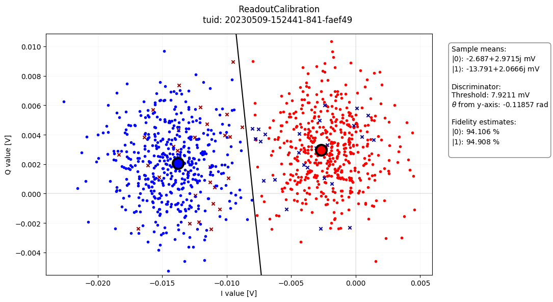
class ReadoutCalibrationAnalysis(dataset=None, tuid=None, label='', settings_overwrite=None, plot_figures=True)[source]#

Bases: BaseAnalysis

Find threshold and angle which discriminates qubit state.

Example

import os


import quantify_core.data.handling as dh
from quantify_core.analysis.readout_calibration_analysis import (
    ReadoutCalibrationAnalysis,
)

# load example data
test_data_dir = "../tests/test_data"
dh.set_datadir(test_data_dir)
ReadoutCalibrationAnalysis(tuid="20230509-152441-841-faef49").run().display_figs_mpl()

analyze_fit_results()[source]#

Check the fit success and populate .quantities_of_interest.

Return type:: None

create_figures()[source]#

Generate figures of interest.

matplotlib figures and axes objects are added to the .figs_mpl and .axs_mpl dictionaries, respectively.

Return type:: None

process_data()[source]#

Process the data so that the analysis can make assumptions on the format.

Return type:: None

run_fitting()[source]#

Fit a state discriminator to the readout calibration data.

Return type:: None

`conditional_oscillation_analysis`#

Module containing an analysis class for the conditional oscillation experiment.

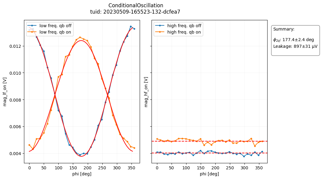
class ConditionalOscillationAnalysis(dataset=None, tuid=None, label='', settings_overwrite=None, plot_figures=True)[source]#

Bases: BaseAnalysis

Analysis class for the conditional oscillation experiment.

For a reference to the conditional oscillation experiment, please see section D in the supplemental material of this paper: https://arxiv.org/abs/1903.02492

Example

from quantify_core.analysis.conditional_oscillation_analysis import (
    ConditionalOscillationAnalysis
)
import quantify_core.data.handling as dh

# load example data
test_data_dir = "../tests/test_data"
dh.set_datadir(test_data_dir)

# run analysis and plot results
analysis = (
    ConditionalOscillationAnalysis(tuid="20230509-165523-132-dcfea7")
    .run()
    .display_figs_mpl()
)

analyze_fit_results()[source]#

Check fit success and populates .quantities_of_interest.

Return type:: None

create_figures()[source]#

Generate figures of interest.

matplolib figures and axes objects are added to the .figs_mpl and .axs_mpl dictionaries., respectively.

Return type:: None

process_data()[source]#

Process the data so that the analysis can make assumptions on the format.

Return type:: None

run_fitting()[source]#

Fit two sinusoidal model to the off/on experiments.

Return type:: None

quantify_core.analysis#

base_analysis#

cosine_analysis#

spectroscopy_analysis#

single_qubit_timedomain#

interpolation_analysis#

optimization_analysis#

fitting_models#

calibration#

readout_calibration_analysis#

conditional_oscillation_analysis#

`quantify_core.analysis`#

`base_analysis`#

`cosine_analysis`#

`spectroscopy_analysis`#

`single_qubit_timedomain`#

`interpolation_analysis`#

`optimization_analysis`#

`fitting_models`#

`calibration`#

`readout_calibration_analysis`#

`conditional_oscillation_analysis`#