Tutorial 3. Building custom analyses - the data analysis framework#

Run an experiment#

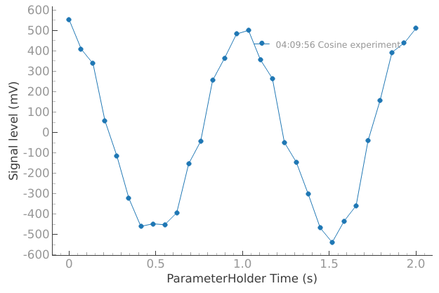
We mock an experiment in order to generate a toy dataset to use in this tutorial.

meas_ctrl = MeasurementControl("meas_ctrl")
plotmon = pqm.PlotMonitor_pyqt("plotmon")
meas_ctrl.instr_plotmon(plotmon.name)
pars = mk_cosine_instrument()

meas_ctrl.settables(pars.t)
meas_ctrl.setpoints(np.linspace(0, 2, 30))
meas_ctrl.gettables(pars.sig)
dataset = meas_ctrl.run("Cosine experiment")

Starting iterative measurement...

plotmon.main_QtPlot

../_images/2bf2d34f42a69dc2d687529915b2a666ffe92ddc970325c56b9412fe0b0d997e.png

Manual analysis steps#

Loading the data#

The Dataset contains all the information required to perform a basic analysis of the experiment. We can alternatively load the dataset from disk based on its TUID, a timestamp-based unique identifier. If you do not know the tuid of the experiment you can find the latest tuid containing a certain string in the experiment name using get_latest_tuid(). See the Data storage documentation for more details on the folder structure and files contained in the data directory.

tuid = get_latest_tuid(contains="Cosine experiment")
dataset = load_dataset(tuid)
dataset

<xarray.Dataset> Size: 480B
Dimensions:  (dim_0: 30)
Coordinates:
    x0       (dim_0) float64 240B 0.0 0.06897 0.1379 0.2069 ... 1.862 1.931 2.0
Dimensions without coordinates: dim_0
Data variables:
    y0       (dim_0) float64 240B 0.4575 0.5193 0.3018 ... 0.3886 0.4622 0.4863
Attributes:
    tuid:                             20241203-040856-789-a20f53
    name:                             Cosine experiment
    grid_2d:                          False
    grid_2d_uniformly_spaced:         False
    1d_2_settables_uniformly_spaced:  False

Performing a fit#

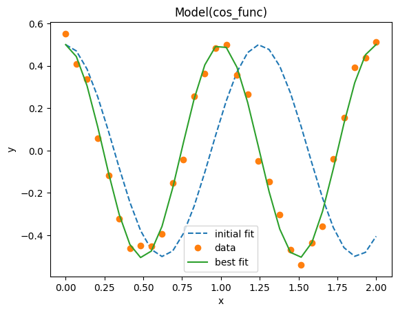
We have a sinusoidal signal in the experiment dataset, the goal is to find the underlying parameters. We extract these parameters by performing a fit to a model, a cosine function in this case. For fitting we recommend using the lmfit library. See the lmfit documentation on how to fit data to a custom model.

# create a fitting model based on a cosine function
fitting_model = lmfit.Model(cos_func)

# specify initial guesses for each parameter
fitting_model.set_param_hint("amplitude", value=0.5, min=0.1, max=2, vary=True)
fitting_model.set_param_hint("frequency", value=0.8, vary=True)
fitting_model.set_param_hint("phase", value=0)
fitting_model.set_param_hint("offset", value=0)
params = fitting_model.make_params()

# here we run the fit
fit_result = fitting_model.fit(dataset.y0.values, x=dataset.x0.values, params=params)

# It is possible to get a quick visualization of our fit using a build-in method of lmfit
_ = fit_result.plot_fit(show_init=True)

../_images/6e63d065dfd0df93ddafd8f41181035bef40ab9f3f1df7c67cc4b517a6ca2a90.png

The summary of the fit result can be nicely printed in a Jupyter-like notebook:

fit_result

Fit Result

Model: Model(cos_func)

Fit Statistics
fitting method	leastsq
# function evals	46
# data points	30
# variables	4
chi-square	0.04818429
reduced chi-square	0.00185324
Akaike info crit.	-185.017590
Bayesian info crit.	-179.412800
R-squared	0.98769060

Parameters
name	value	standard error	relative error	initial value	min	max	vary
frequency	1.00258074	0.00695386	(0.69%)	0.8	-inf	inf	True
amplitude	0.49951199	0.01100843	(2.20%)	0.5	0.10000000	2.00000000	True
offset	0.00321185	0.00850590	(264.83%)	0	-inf	inf	True
phase	0.01574456	0.04905609	(311.57%)	0	-inf	inf	True

Correlations (unreported values are < 0.100)
Parameter1	Parameter 2	Correlation
frequency	phase	-0.8869
frequency	offset	-0.3795
offset	phase	+0.3373
frequency	amplitude	-0.1144
amplitude	phase	+0.1024

Analyzing the fit result and saving key quantities#

quantities_of_interest = {
    "amplitude": fit_result.params["amplitude"].value,
    "frequency": fit_result.params["frequency"].value,
}
quantities_of_interest

{'amplitude': np.float64(0.49951199388976786),
 'frequency': np.float64(1.002580739296254)}

Now that we have the relevant quantities, we want to store them in the same experiment directory where the raw dataset is stored.

First, we determine the experiment directory on the file system.

# the experiment folder is retrieved with a convenience function
exp_folder = Path(locate_experiment_container(dataset.tuid))
exp_folder

PosixPath('/root/quantify-data/20241203/20241203-040856-789-a20f53-Cosine experiment')

Then, we save the quantities of interest to disk in the human-readable JSON format.

with open(exp_folder / "quantities_of_interest.json", "w", encoding="utf-8") as file:
    json.dump(quantities_of_interest, file)

Plotting and saving figures#

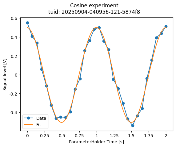
We would like to save a plot of our data and the fit in our lab logbook but the figure above is not fully satisfactory: there are no units and no reference to the original dataset.

Below we create our own plot for full control over the appearance and we store it on disk in the same experiment directory. For plotting, we use the ubiquitous matplotlib and some visualization utilities.

# create matplotlib figure
fig, ax = plt.subplots()

# plot data
dataset.y0.plot.line(ax=ax, x="x0", marker="o", label="Data")

# plot fit
x_fit = np.linspace(dataset["x0"][0].values, dataset["x0"][-1].values, 1000)
y_fit = cos_func(x=x_fit, **fit_result.best_values)
ax.plot(x_fit, y_fit, label="Fit")
ax.legend()

# set units-aware tick labels
set_xlabel(dataset.x0.long_name, dataset.x0.units)
set_ylabel(dataset.y0.long_name, dataset.y0.units)

# add a reference to the origal dataset in the figure title
fig.suptitle(f"{dataset.attrs['name']}\ntuid: {dataset.attrs['tuid']}")

# Save figure
fig.savefig(exp_folder / "Cosine fit.png", dpi=300, bbox_inches="tight")

../_images/c67d80e0327e89b588cb4342d7b27ea63d76e10f49f16679f7bb7c32564a7c00.png

Reusable fitting model and analysis steps#

The previous steps achieve our goal, however, the code above is not easily reusable and hard to maintain or debug. We can do better than this! We can package our code in functions that perform specific tasks. In addition, we will use the objected-oriented interface of lmfit to further structure our code. We explore the details of the object-oriented approach later in this tutorial.

class MyCosineModel(lmfit.model.Model):
    """
    `lmfit` model with a guess for a cosine fit.
    """

    def __init__(self, *args, **kwargs):
        """Configures the constraints of the model."""
        # pass in the model's equation
        super().__init__(cos_func, *args, **kwargs)

        # configure constraints that are independent from the data to be fitted

        self.set_param_hint("frequency", min=0, vary=True)  # enforce positive frequency
        self.set_param_hint("amplitude", min=0, vary=True)  # enforce positive amplitude
        self.set_param_hint("offset", vary=True)
        self.set_param_hint(
            "phase", vary=True, min=-np.pi, max=np.pi
        )  # enforce phase range

    def guess(self, data, **kws) -> lmfit.parameter.Parameters:
        """Guess parameters based on the data."""

        self.set_param_hint("offset", value=np.average(data))
        self.set_param_hint("amplitude", value=(np.max(data) - np.min(data)) / 2)
        # a simple educated guess based on experiment type
        # a more elaborate but general approach is to use a Fourier transform
        self.set_param_hint("frequency", value=1.2)

        params_ = self.make_params()
        return lmfit.models.update_param_vals(params_, self.prefix, **kws)

Most of the code related to the fitting model is now packed in a single object, while the analysis steps are split into functions that take care of specific tasks.

def extract_data(label: str) -> xr.Dataset:
    """Loads a dataset from its label."""
    tuid_ = get_latest_tuid(contains=label)
    dataset_ = load_dataset(tuid_)
    return dataset_


def run_fitting(dataset_: xr.Dataset) -> lmfit.model.ModelResult:
    """Executes fitting."""
    model = MyCosineModel()  # create the fitting model
    params_guess = model.guess(data=dataset_.y0.values)
    result = model.fit(
        data=dataset_.y0.values, x=dataset_.x0.values, params=params_guess
    )
    return result


def analyze_fit_results(fit_result_: lmfit.model.ModelResult) -> dict:
    """Analyzes the fit results and saves quantities of interest."""
    quantities = {
        "amplitude": fit_result_.params["amplitude"].value,
        "frequency": fit_result_.params["frequency"].value,
    }
    return quantities


def plot_fit(
    fig_: matplotlib.figure.Figure,
    ax_: matplotlib.axes.Axes,
    dataset_: xr.Dataset,
    fit_result_: lmfit.model.ModelResult,
) -> Tuple[matplotlib.figure.Figure, matplotlib.axes.Axes]:
    """Plots a fit result."""
    dataset_.y0.plot.line(ax=ax_, x="x0", marker="o", label="Data")  # plot data

    x_fit_ = np.linspace(dataset_["x0"][0].values, dataset_["x0"][-1].values, 1000)
    y_fit_ = cos_func(x=x_fit_, **fit_result_.best_values)
    ax_.plot(x_fit, y_fit_, label="Fit")  # plot fit
    ax_.legend()

    # set units-aware tick labels
    set_xlabel(dataset_.x0.long_name, dataset_.x0.units, ax_)
    set_ylabel(dataset_.y0.long_name, dataset_.y0.units, ax_)

    # add a reference to the original dataset_ in the figure title
    fig_.suptitle(f"{dataset_.attrs['name']}\ntuid: {dataset_.attrs['tuid']}")


def save_quantities_of_interest(tuid_: str, quantities_of_interest_: dict) -> None:
    """Saves the quantities of interest to disk in JSON format."""
    exp_folder_ = Path(locate_experiment_container(tuid_))
    # Save fit results
    with open(exp_folder_ / "quantities_of_interest.json", "w", encoding="utf-8") as f_:
        json.dump(quantities_of_interest_, f_)


def save_mpl_figure(tuid_: str, fig_: matplotlib.figure.Figure) -> None:
    """Saves a matplotlib figure as PNG."""
    exp_folder_ = Path(locate_experiment_container(tuid_))
    fig_.savefig(exp_folder_ / "Cosine fit.png", dpi=300, bbox_inches="tight")
    plt.close(fig_)

Now the execution of the entire analysis becomes much more readable and clean:

dataset = extract_data(label="Cosine experiment")
fit_result = run_fitting(dataset)
quantities_of_interest = analyze_fit_results(fit_result)
save_quantities_of_interest(dataset.tuid, quantities_of_interest)
fig, ax = plt.subplots()
plot_fit(fig_=fig, ax_=ax, dataset_=dataset, fit_result_=fit_result)
save_mpl_figure(dataset.tuid, fig)

If we inspect the experiment directory, we will find a structure that looks like the following:

20230125-172712-018-87b9bf-Cosine experiment/
├── Cosine fit.png
├── dataset.hdf5
├── quantities_of_interest.json
└── snapshot.json

Creating a simple analysis class#

Even though we have improved code structure greatly, in order to execute the same analysis against some other dataset we would have to copy-paste a significant portion of code (the analysis steps).

We tackle this by taking advantage of the Object Oriented Programming (OOP) in python. We will create a python class that serves as a structured container for data (attributes) and the methods (functions) that act on the information.

Some of the advantages of OOP are:

the same class can be instantiated multiple times to act on different data while reusing the same methods;
all the methods have access to all the data (attributes) associated with a particular instance of the class;
subclasses can inherit from other classes and extend their functionalities.

Let’s now observe what such a class could look like.

Warning

This analysis class is intended for educational purposes only. It is not intended to be used as a template! See the end of the tutorial for the recommended usage of the analysis framework.

class MyCosineAnalysis:
    """Analysis as a class."""

    def __init__(self, label: str):
        """This is a special method that python calls when an instance of this class is
        created."""

        self.label = label

        # objects to be filled up later when running the analysis
        self.tuid = None
        self.dataset = None
        self.fit_results = {}
        self.quantities_of_interest = {}
        self.figs_mpl = {}
        self.axs_mpl = {}

    # with just slight modification our functions become methods
    # with the advantage that we have access to all the necessary information from self
    def run(self):
        """Execute the analysis steps."""
        self.extract_data()
        self.run_fitting()
        self.analyze_fit_results()
        self.create_figures()
        self.save_quantities_of_interest()
        self.save_figures()

    def extract_data(self):
        """Load data from disk."""
        self.tuid = get_latest_tuid(contains=self.label)
        self.dataset = load_dataset(tuid)

    def run_fitting(self):
        """Fits the model to the data."""
        model = MyCosineModel()
        guess = model.guess(self.dataset.y0.values)
        result = model.fit(
            self.dataset.y0.values, x=self.dataset.x0.values, params=guess
        )
        self.fit_results.update({"cosine": result})

    def analyze_fit_results(self):
        """Analyzes the fit results and saves quantities of interest."""
        self.quantities_of_interest.update(
            {
                "amplitude": self.fit_results["cosine"].params["amplitude"].value,
                "frequency": self.fit_results["cosine"].params["frequency"].value,
            }
        )

    def save_quantities_of_interest(self):
        """Save quantities of interest to disk."""
        exp_folder_ = Path(locate_experiment_container(self.tuid))
        with open(
            exp_folder_ / "quantities_of_interest.json", "w", encoding="utf-8"
        ) as file_:
            json.dump(self.quantities_of_interest, file_)

    def plot_fit(self, fig_: matplotlib.figure.Figure, ax_: matplotlib.axes.Axes):
        """Plot the fit result."""

        self.dataset.y0.plot.line(ax=ax_, x="x0", marker="o", label="Data")  # plot data

        x_fit_ = np.linspace(
            self.dataset["x0"][0].values, self.dataset["x0"][-1].values, 1000
        )
        y_fit_ = cos_func(x=x_fit_, **self.fit_results["cosine"].best_values)
        ax_.plot(x_fit_, y_fit_, label="Fit")  # plot fit
        ax_.legend()

        # set units-aware tick labels
        set_xlabel(self.dataset.x0.long_name, self.dataset.x0.attrs["units"], ax_)
        set_ylabel(self.dataset.y0.long_name, self.dataset.y0.attrs["units"], ax_)

        # add a reference to the original dataset in the figure title
        fig_.suptitle(f"{dataset.attrs['name']}\ntuid: {dataset.attrs['tuid']}")

    def create_figures(self):
        """Create figures."""
        fig_, ax_ = plt.subplots()
        self.plot_fit(fig_, ax_)

        fig_id = "cos-data-and-fit"
        self.figs_mpl.update({fig_id: fig_})
        # keep a reference to `ax` as well
        # it can be accessed later to apply modifications (e.g., in a notebook)
        self.axs_mpl.update({fig_id: ax_})

    def save_figures(self):
        """Save figures to disk."""
        exp_folder_ = Path(locate_experiment_container(self.tuid))
        for fig_name, fig_ in self.figs_mpl.items():
            fig_.savefig(exp_folder_ / f"{fig_name}.png", dpi=300, bbox_inches="tight")
            plt.close(fig_)

Running the analysis is now as simple as:

a_obj = MyCosineAnalysis(label="Cosine experiment")
a_obj.run()
a_obj.figs_mpl["cos-data-and-fit"]

The first line will instantiate the class by calling the .__init__() method.

As expected this will save similar files into the experiment directory:

20230125-172712-018-87b9bf-Cosine experiment/
├── cos-data-and-fit.png
├── Cosine fit.png
├── dataset.hdf5
├── quantities_of_interest.json
└── snapshot.json

Extending the BaseAnalysis#

While the above stand-alone class provides the gist of an analysis, we can do even better by defining a structured framework that all analyses need to adhere to and factoring out the pieces of code that are common to most analyses. Besides that, the overall functionality can be improved.

Here is where the BaseAnalysis enters the scene. It allows us to focus only on the particular aspect of our custom analysis by implementing only the relevant methods. Take a look at how the above class is implemented where we are making use of the analysis framework. For completeness, a fully documented CosineModel which can serve as a template is shown as well.

display_source_code(CosineModel)
display_source_code(CosineAnalysis)

class CosineModel(lmfit.model.Model):
    """
    Exemplary lmfit model with a guess for a cosine.

    .. note::

        The :mod:`lmfit.models` module provides several fitting models that might fit
        your needs out of the box.
    """

    def __init__(self, *args, **kwargs):
        # pass in the model's equation
        super().__init__(cos_func, *args, **kwargs)

        # configure constraints that are independent from the data to be fitted
        self.set_param_hint("frequency", min=0, vary=True)  # enforce positive frequency
        self.set_param_hint("amplitude", min=0, vary=True)  # enforce positive amplitude
        self.set_param_hint("offset", vary=True)
        self.set_param_hint(
            "phase", vary=True, min=-np.pi, max=np.pi
        )  # enforce phase range

    # pylint: disable=missing-function-docstring
    def guess(self, data, x, **kws) -> lmfit.parameter.Parameters:
        """
        guess parameters based on the data

        Parameters
        ----------
        data: np.ndarray
            Data to fit to
        x: np.ndarray
            Independet variable
        """

        self.set_param_hint("offset", value=np.average(data))
        self.set_param_hint("amplitude", value=(np.max(data) - np.min(data)) / 2)

        # Guess frequency and phase using Fourier Transform
        freq_guess, phase_guess = fft_freq_phase_guess(data, x)
        phase_wrap = (phase_guess + np.pi) % (2 * np.pi) - np.pi
        self.set_param_hint("frequency", value=freq_guess)
        self.set_param_hint("phase", value=phase_wrap)

        params = self.make_params()
        return lmfit.models.update_param_vals(params, self.prefix, **kws)

    # Same design patter is used in lmfit.models to inherit common docstrings.
    # We adjust these common docstrings to our docs build pipeline
    __init__.__doc__ = get_model_common_doc() + mk_seealso("cos_func")
    guess.__doc__ = get_guess_common_doc()

class CosineAnalysis(ba.BaseAnalysis):
    """
    Exemplary analysis subclass that fits a cosine to a dataset.
    """

    def process_data(self):
        """
        In some cases, you might need to process the data, e.g., reshape, filter etc.,
        before starting the analysis. This is the method where it should be done.

        See :meth:`~quantify_core.analysis.spectroscopy_analysis.ResonatorSpectroscopyAnalysis.process_data`
        for an implementation example.
        """  # pylint: disable=line-too-long

    def run_fitting(self):
        """
        Fits a :class:`~quantify_core.analysis.fitting_models.CosineModel` to the data.
        """
        # create a fitting model based on a cosine function
        model = CosineModel()
        guess = model.guess(self.dataset.y0.values, x=self.dataset.x0.values)
        result = model.fit(
            self.dataset.y0.values, x=self.dataset.x0.values, params=guess
        )
        self.fit_results.update({"cosine": result})

    def create_figures(self):
        """
        Creates a figure with the data and the fit.
        """
        fig, ax = plt.subplots()
        fig_id = "cos_fit"
        self.figs_mpl.update({fig_id: fig})
        self.axs_mpl.update({fig_id: ax})

        self.dataset.y0.plot(ax=ax, x="x0", marker="o", linestyle="")
        qpl.plot_fit(ax, self.fit_results["cosine"])
        qpl.plot_textbox(ax, ba.wrap_text(self.quantities_of_interest["fit_msg"]))

        adjust_axeslabels_SI(ax)
        qpl.set_suptitle_from_dataset(fig, self.dataset, "x0-y0")
        ax.legend()

    def analyze_fit_results(self):
        """
        Checks fit success and populates :code:`quantities_of_interest`.
        """
        fit_result = self.fit_results["cosine"]
        fit_warning = ba.check_lmfit(fit_result)

        # If there is a problem with the fit, display an error message in the text box.
        # Otherwise, display the parameters as normal.
        if fit_warning is None:
            self.quantities_of_interest["fit_success"] = True
            unit = self.dataset.y0.units
            text_msg = "Summary\n"
            text_msg += format_value_string(
                r"$f$", fit_result.params["frequency"], end_char="\n", unit="Hz"
            )
            text_msg += format_value_string(
                r"$A$", fit_result.params["amplitude"], unit=unit
            )
        else:
            text_msg = fit_warning
            self.quantities_of_interest["fit_success"] = False

        # save values and fit uncertainty
        for parameter_name in ["frequency", "amplitude"]:
            self.quantities_of_interest[parameter_name] = ba.lmfit_par_to_ufloat(
                fit_result.params[parameter_name]
            )
        self.quantities_of_interest["fit_msg"] = text_msg

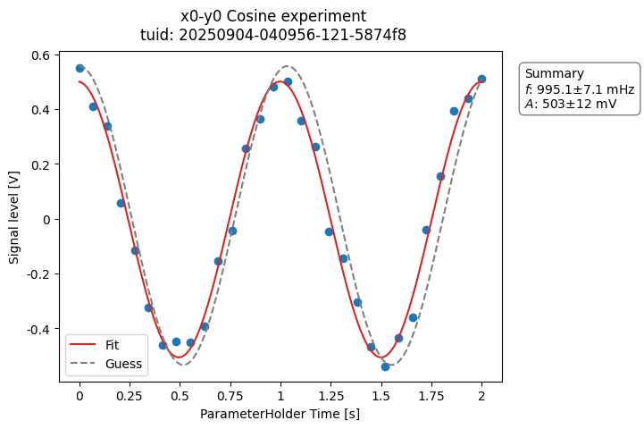
Now we can simply execute it against our latest experiment as follows:

a_obj = CosineAnalysis(label="Cosine experiment").run()
a_obj.display_figs_mpl()

../_images/e889d48042667f9aba3aeddf1160d6634be60c591dd841abaf37a5a797239648.png

Inspecting the experiment directory will show something like this:

20230125-172712-018-87b9bf-Cosine experiment/
├── analysis_CosineAnalysis/
│   ├── dataset_processed.hdf5
│   ├── figs_mpl/
│   │   ├── cos_fit.png
│   │   └── cos_fit.svg
│   ├── fit_results/
│   │   └── cosine.txt
│   └── quantities_of_interest.json
├── cos-data-and-fit.png
├── Cosine fit.png
├── dataset.hdf5
├── quantities_of_interest.json
└── snapshot.json

As you can conclude from the CosineAnalysis code, we did not implement quite a few methods in there. These are provided by the BaseAnalysis. To gain some insight into what exactly is being executed we can enable the logging module and use the internal logger of the analysis instance:

# activate logging and set global level to show warnings only
logging.basicConfig(level=logging.WARNING)

# set analysis logger level to info (the logger is inherited from BaseAnalysis)
a_obj.logger.setLevel(level=logging.INFO)
_ = a_obj.run()

INFO:CosineAnalysis:Executing `.analysis_steps` of CosineAnalysis

INFO:CosineAnalysis:extracting data: <bound method BaseAnalysis.extract_data of <quantify_core.analysis.cosine_analysis.CosineAnalysis object at 0x793b153a3820>>

INFO:CosineAnalysis:executing step 1: <bound method CosineAnalysis.process_data of <quantify_core.analysis.cosine_analysis.CosineAnalysis object at 0x793b153a3820>>

INFO:CosineAnalysis:executing step 2: <bound method CosineAnalysis.run_fitting of <quantify_core.analysis.cosine_analysis.CosineAnalysis object at 0x793b153a3820>>

INFO:CosineAnalysis:executing step 3: <bound method CosineAnalysis.analyze_fit_results of <quantify_core.analysis.cosine_analysis.CosineAnalysis object at 0x793b153a3820>>

INFO:CosineAnalysis:executing step 4: <bound method CosineAnalysis.create_figures of <quantify_core.analysis.cosine_analysis.CosineAnalysis object at 0x793b153a3820>>

INFO:CosineAnalysis:executing step 5: <bound method BaseAnalysis.adjust_figures of <quantify_core.analysis.cosine_analysis.CosineAnalysis object at 0x793b153a3820>>

INFO:CosineAnalysis:executing step 6: <bound method BaseAnalysis.save_figures of <quantify_core.analysis.cosine_analysis.CosineAnalysis object at 0x793b153a3820>>

INFO:CosineAnalysis:executing step 7: <bound method BaseAnalysis.save_quantities_of_interest of <quantify_core.analysis.cosine_analysis.CosineAnalysis object at 0x793b153a3820>>

INFO:CosineAnalysis:executing step 8: <bound method BaseAnalysis.save_processed_dataset of <quantify_core.analysis.cosine_analysis.CosineAnalysis object at 0x793b153a3820>>

INFO:CosineAnalysis:executing step 9: <bound method BaseAnalysis.save_fit_results of <quantify_core.analysis.cosine_analysis.CosineAnalysis object at 0x793b153a3820>>