Tutorial 4. Adaptive Measurements#
See also
The complete source code of this tutorial can be found in
This tutorial requires familiarity with the core concepts of Quantify. We highly recommended to read the user guide and follow Tutorial 1. Controlling a basic experiment using MeasurementControl and Tutorial 2. Advanced capabilities of the MeasurementControl first.
In this tutorial, we explore the adaptive functionality of the MeasurementControl.
With this mode, instead of predefining a grid of values to sweep through, we provide an optimization function and an initial state to the meas_ctrl.
The meas_ctrl will then use this function to build the sweep. We import our usual modules and set up a meas_ctrl with visualization:
Before instantiating any instruments or starting a measurement we change the
directory in which the experiments are saved using the
set_datadir()
[get_datadir()] functions.
⚠️ Warning!
We recommend always setting the directory at the start of the python kernel and stick to a single common data directory for all notebooks/experiments within your measurement setup/PC.
The cell below sets a default data directory (~/quantify-data on Linux/macOS or
$env:USERPROFILE\\quantify-data on Windows) for tutorial purposes. Change it to your
desired data directory. The utilities to find/search/extract data only work if
all the experiment containers are located within the same directory.
set_datadir(default_datadir())
Data will be saved in:
/root/quantify-data
meas_ctrl = MeasurementControl("meas_ctrl")
insmon = InstrumentMonitor("InstrumentMonitor")
plotmon = pqm.PlotMonitor_pyqt("plotmon_meas_ctrl")
meas_ctrl.instr_plotmon(plotmon.name)
Finding a minimum#
We will create a mock Instrument our meas_ctrl will interact with. In this case, it is a simple parabola centered at the origin.
para = Instrument("parabola")

para.add_parameter("x", unit="m", label="X", parameter_class=ManualParameter)
para.add_parameter("y", unit="m", label="Y", parameter_class=ManualParameter)

para.add_parameter(
    "noise", unit="V", label="white noise amplitude", parameter_class=ManualParameter
)
para.add_parameter(
    "acq_delay", initial_value=0.1, unit="s", parameter_class=ManualParameter
)


def _amp_model():
    time.sleep(
        para.acq_delay()
    )  # for display purposes, just so we can watch the live plot update
    return para.x() ** 2 + para.y() ** 2 + para.noise() * np.random.rand(1)


para.add_parameter("amp", unit="V", label="Amplitude", get_cmd=_amp_model)
<qcodes.parameters.parameter.Parameter: amp at 140051342302704>
Next, we will use the optimize package from scipy to provide our adaptive function.
You can of course implement your own functions for this purpose, but for brevity we will use something standard and easily available.
Then, we set our Settables and Gettables as usual, and define a new dictionary af_pars.
The only required key in this object is adaptive_function, the value to be used by the adaptive function.
The remaining fields in this dictionary are the arguments to the adaptive function itself. We also add some noise into the parabola to stress our adaptive function.
As such, it is highly recommended to thoroughly read the documentation around the adaptive function you are using.
We will use the optimize.minimize function (note this is passed by reference as opposed to calling the minimize function), which requires an initial state named "x0" and an algorithm to use named "method".
In this case, we are starting at [-50, -50] and hope to minimize these values relative to our parabola function.
Of course, this parabola has its global minimum at the origin, thus these values will tend towards 0 as our algorithm progresses.
meas_ctrl.settables([para.x, para.y])
af_pars = {
    "adaptive_function": optimize.minimize,  # used by meas_ctrl
    "x0": [-50, -50],  # used by `optimize.minimize` (in this case)
    "method": "Nelder-Mead",  # used by `optimize.minimize` (in this case)
    "options": {"maxfev": 100},  # limit the maximum evaluations of the gettable(s)
}
para.noise(0.5)
meas_ctrl.gettables(para.amp)
dset = meas_ctrl.run_adaptive("nelder_mead_optimization", af_pars)
dset
<xarray.Dataset> Size: 2kB
Dimensions:  (dim_0: 100)
Coordinates:
    x0       (dim_0) float64 800B -50.0 -52.5 -50.0 ... -0.02341 -0.02341
    x1       (dim_0) float64 800B -50.0 -50.0 -52.5 ... 0.05432 0.05441 0.05434
Dimensions without coordinates: dim_0
Data variables:
    y0       (dim_0) float64 800B 5e+03 5.257e+03 5.256e+03 ... 0.2194 0.2416
Attributes:
    tuid:                             20250904-041007-422-6e95db
    name:                             nelder_mead_optimization
    grid_2d:                          False
    grid_2d_uniformly_spaced:         False
1d_2_settables_uniformly_spaced: Trueplotmon.main_QtPlot
plotmon.secondary_QtPlot

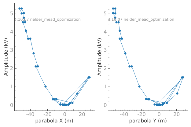
We can see from the graphs that the values of the settables in the dataset snake towards 0 as expected. Success!
Analysis#
There are several analysis classes available in quantify-core that can be used to visualize and extract relevant information from the results of these adaptive measurements.
The OptimizationAnalysis class searches the dataset for the optimal datapoint and provides a number of useful plots to visualize the convergence of the measurement result around the minimum.
a_obj = oa.OptimizationAnalysis(dset)
a_obj.run()
a_obj.display_figs_mpl()
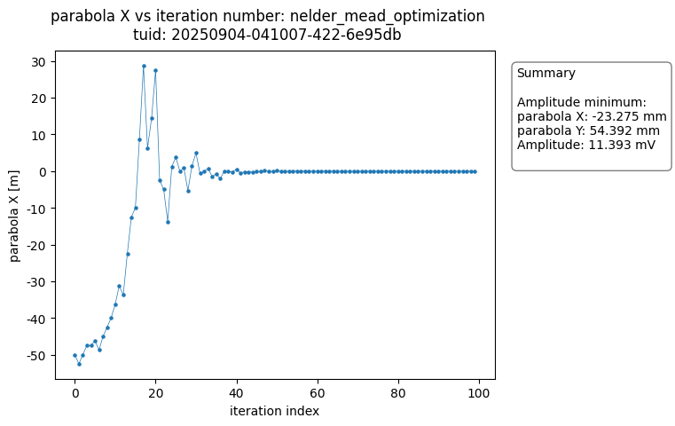
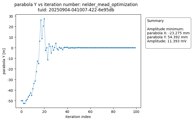
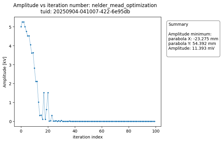
The analysis generates plots of each of the variables versus the number of iteration steps completed. The figures show the data converging on the optimal value.
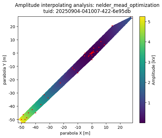
The InterpolationAnalysis2D class can be used to generate a 2-dimensional heatmap that interpolates between a set of irregularly spaced datapoints.
a_obj = InterpolationAnalysis2D(dset)
a_obj.run()
a_obj.display_figs_mpl()
Adaptive Sampling#
Quantify is designed to be modular and the adaptive functions support is no different. To this end, the meas_ctrl has first-class support for the adaptive package.
Let’s see what the same experiment looks like with this module. Note the fields of the af_pars dictionary have changed to be compatible with the different adaptive functions that we are using.
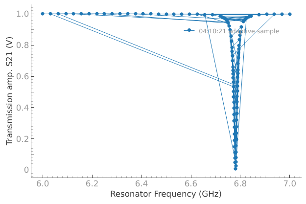
As a practical example, let’s revisit a Resonator Spectroscopy experiment. This time we only know our device has a resonance in 6-7 GHz range. We really don’t want to sweep through a million points, so instead let’s use an adaptive sampler to quickly locate our peak.
res = Instrument("Resonator")

res.add_parameter("freq", unit="Hz", label="Frequency", parameter_class=ManualParameter)
res.add_parameter("amp", unit="V", label="Amplitude", parameter_class=ManualParameter)
_fwhm = 15e6  # pretend you don't know what this value is
_res_freq = 6.78e9  # pretend you don't know what this value is
_noise_level = 0.1


def lorenz():
    """A Lorenz model function."""
    time.sleep(0.02)  # for display purposes, just so we can watch the graph update
    return (
        1
        - (
            res.amp()
            * ((_fwhm / 2.0) ** 2)
            / ((res.freq() - _res_freq) ** 2 + (_fwhm / 2.0) ** 2)
        )
        + _noise_level * np.random.rand(1)
    )


res.add_parameter("S21", unit="V", label="Transmission amp. S21", get_cmd=lorenz)
<qcodes.parameters.parameter.Parameter: S21 at 140051326734144>
_noise_level = 0.0
res.amp(1)
meas_ctrl.settables([res.freq])
af_pars = {
    "adaptive_function": adaptive.learner.Learner1D,
    "goal": lambda l: l.npoints > 99,
    "bounds": (6.0e9, 7.0e9),
}
meas_ctrl.gettables(res.S21)
dset = meas_ctrl.run_adaptive("adaptive sample", af_pars)
dset
<xarray.Dataset> Size: 2kB
Dimensions:  (dim_0: 100)
Coordinates:
    x0       (dim_0) float64 800B 6e+09 7e+09 6.5e+09 ... 6.77e+09 6.754e+09
Dimensions without coordinates: dim_0
Data variables:
    y0       (dim_0) float64 800B 0.9999 0.9988 0.9993 ... 0.6186 0.6391 0.9237
Attributes:
    tuid:                             20250904-041021-472-9804ea
    name:                             adaptive sample
    grid_2d:                          False
    grid_2d_uniformly_spaced:         False
1d_2_settables_uniformly_spaced: Trueplotmon.main_QtPlot
FAQ#
Can I return multi-dimensional data from a Gettable in Adaptive Mode?#
Yes, but only the first dimension (y0) will be considered by the adaptive function;
the remaining dimensions will merely be saved to the dataset.